Experience of tuning Llama3 405B on AMD MI300x

Introduction

AMD GPUs, and especially the MI300X series, are a serious alternative to NVIDIA AI hardware, providing more performance per dollar invested. Our system consisted of a single node with 8 AMD MI300x GPUs, and for fine-tuning, we used JAX. In this article, we will tell the whole story of fine-tuning LLaMA 405B, including details of parameter sharding and LoRA implementation.

What is JAX and why we chose it

JAX is a powerful machine learning library that combines NumPy-like APIs, automatic differentiation, and the Google XLA compiler. It has excellent APIs for model parallelism, making it ideal for training huge models like LLaMA 3.1 405B.

Why I love JAX:

1. Pure functions: JAX motivates writing pure functions (if you want to compile code using JIT), which simplifies composition, debugging, and reading of code.

2. Advanced parallelism: JAX's flexible JIT API library natively supports advanced data and model parallelism, which is crucial for large-scale training.

3. Improving codebase cleanliness: JAX's design philosophy encourages writing code that is natively portable across hardware platforms (CPU, GPU, TPU), leading to cleaner and more maintainable codebases.

If you want to delve deeper into the advantages of JAX over PyTorch, I recommend reading the post PyTorch is dead. Long live JAX.

JAX is especially remarkable when working with non-NVIDIA hardware:

When working with AMD, JAX provides numerous advantages:

1. Hardware-independent approach: JAX uses the XLA (Accelerated Linear Algebra) compiler, which compiles computations into a hardware-independent intermediate representation (HLO graph). This allows optimizing and efficiently executing the same JAX code on different hardware backends, including AMD GPUs, without modifications.

2. Platform-independent optimizations: The XLA compiler performs optimizations regardless of the hardware, benefiting all supported platforms.

3. Simplified portability: When working with JAX, switching from NVIDIA to AMD (or other supported hardware) requires only minimal code changes. This is significantly different from PyTorch, which is more closely tied to the NVIDIA CUDA ecosystem.
   

   • PyTorch often uses CUDA-specific implementations (e.g., torch.cuda calls, scaled_dot_product_attention).

   • Although PyTorch supports other backends like ROCm for AMD GPUs, porting code can be challenging due to NVIDIA-specific code execution paths.

   • The process of "getting rid of NVIDIA" in PyTorch code can increase complexity and hinder portability.

Preparing JAX for AMD is extremely simple!

Setting up JAX on AMD GPUs is a very straightforward process:

# Pull the Docker image:
docker pull rocm/jax:latest

# Run the Docker container:
docker run -it -w /workspace --device=/dev/kfd --device=/dev/dri --group-add video --cap-add=SYS_PTRACE --security-opt seccomp=unconfined --shm-size 16G rocm/jax:latest

# Verify the installation:
python3 -c 'import jax; print(jax.devices())'

I worked with an AMD node consisting of 8 AMD MI300x GPUs. Each MI300x had 192 GB of HBM3 memory. They perform extremely well compared to the new NVIDIA H100 GPUs. (See comparison below, source: TensorWave)

Training LLaMA 405B: Performance and Scalability

Using JAX, I was able to train the LLaMA 405B model on AMD GPUs, achieving impressive results.

We performed fine-tuning LoRA with all model weights and lora parameters with bfloat16 precision, with LoRA rank = 8 and LoRA alpha = 16:

• Model size: LLaMA model weights occupy approximately 800 GB VRAM.

• LoRA weights + optimizer state: approximately 400 GB VRAM.

• Total VRAM usage: 77% of total VRAM, approximately 1200 GB.

• Limitations: due to the large size of the 405B model, space for batch sizes and sequence lengths was limited. I used a batch size of 16 and a sequence length of 64.

• JIT compilation: additionally, due to space constraints, I was unable to run the JIT-compiled version; it likely requires slightly more space than the eager mode graph.

• Training speed: approximately 35 tokens per second in JAX eager mode (1 training step took 30 s)

• Memory efficiency: consistently around 70%

• Scalability: when working with JAX, scalability was approximately linear across all 8 GPUs.

Below are the GPU utilization, memory efficiency, and rocm-smi results for 8 GPUs on one fine-tuning training step:

• GPU utilization:

  

• VRAM usage:

  

results of rocm-smi:

Full information on GPU usage, VRAM, and rocm-smi data can be found in our Github repository.

Our training system

We have ported the LLaMA 3.1 architecture from PyTorch to JAX. Our implementation can be studied in the GitHub repository.

This port has opened up new possibilities for us in terms of performance and scalability.

Model loading and sharding parameters

To work with a model as large as LLaMA 405B, efficient parameter sharding across multiple devices is required. Below we will explain how we achieved this using JAX.

Sharding parameters in JAX

To efficiently distribute the large LLaMA 405B model across 8 AMD GPUs, we applied the JAX device mesh function (codepointer). The device mesh arranges the available devices into a multi-dimensional grid, allowing us to specify how computations and data will be partitioned. In our system, we created a mesh with the shape (1, 8, 1), with axes such as data parallelism (dp), fully sharded data parallelism (fsdp), and model parallelism (mp). We then applied specific sharding rules to the model parameters, specifying for each model tensor how its dimensions would be split across the mesh axes.

DEVICES = jax.devices()
DEVICE_COUNT = len(DEVICES)
DEVICE_MESH = mesh_utils.create_device_mesh((1, 8, 1))
MESH = Mesh(devices=DEVICE_MESH, axis_names=("dp", "fsdp", "mp"))

Sharding visualization

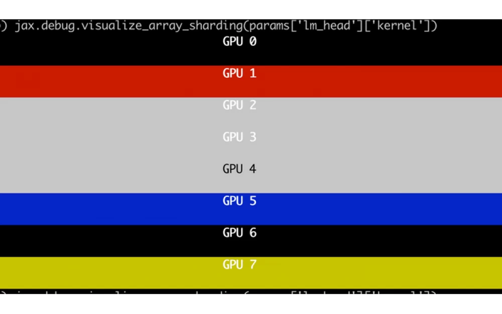
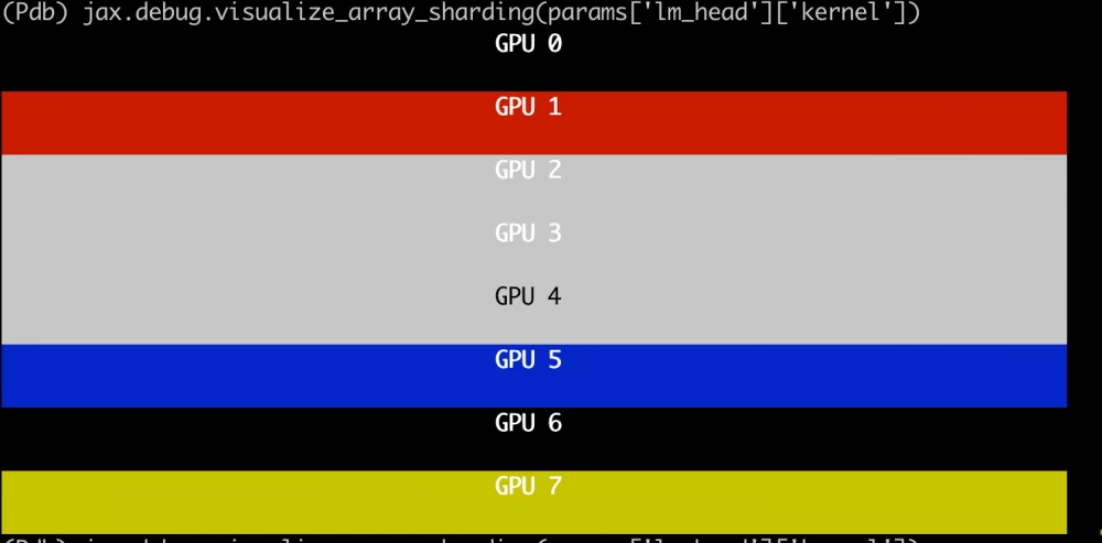
Array sharding can be visualized using jax.debug.visualize_array_sharding. This is incredibly useful for verifying the correct application of sharding specifications.

Sharding rules

We have defined sharding rules for various model components:

Parameter Sharding Method

• Regular Parameters: sharded across 8 GPUs.
  

  • For example, the LM head tensor (lm_head/kernel) has two axes, sharded with PS("fsdp", "mp"); in our case, this is 8, 1, so we see that the tensor is sharded across 8 GPUs along the first axis.

  • 

• Unreplicated Parameters:
  

  • Parameters without sharding specifications are replicated across all devices.

  • For example, layer norms (attention_norm/kernel and ffn_norm/kernel) use PS(None).

    Read also:

    • 5 single-board PCs for various tasks: November news

    

Applying Sharding Constraints

During model loading, we incrementally shard the model weights using special sharding functions:

def make_shard_and_gather_fns(partition_specs):
    def make_shard_fn(partition_spec):
        out_sharding = NamedSharding(mesh, partition_spec)
        def shard_fn(tensor):
            return jax.device_put(tensor, out_sharding).block_until_ready()
        return shard_fn

    shard_fns = jax.tree_util.tree_map(make_shard_fn, partition_specs)
    return shard_fns

# Create sharding functions based on partitioning rules
shard_fns = make_shard_and_gather_fns(partitioning_rules)

This allows us to place each parameter on the appropriate devices with the specified sharding.

Training Batch Sharding

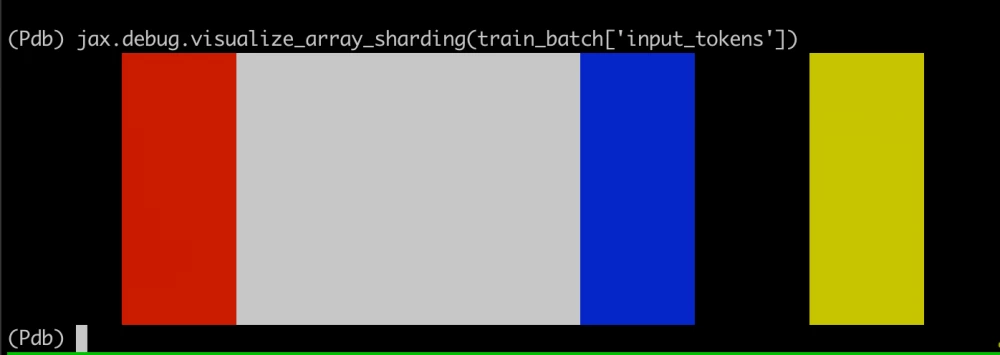
Initially, the training batch is created in the usual way. Before passing it to the model, we shard it across GPUs according to the following code:

train_batch = jax.device_put(
    train_batch, NamedSharding(self.mesh, PS("dp", "fsdp"))
)

Here we specify that the training batch should be sharded between the data parallel ("dp") and fully sharded data parallel ("fsdp") axes, which in our case correspond to 1, 8; this leads to the following visualization:

• before sharding

  

• after calling jax.device_put

  

LoRA Training Implementation

LoRA (Low-Rank Adaptation) reduces the number of parameters for training by breaking down weight updates into low-rank matrices. This is especially useful for fine-tuning large models.

Key aspects of our LoRA implementation:

1. Separate parameterization: we store LoRA parameters (lora_a and lora_b) separately from the main model parameters.

2. Gradient stopping: we use jax.lax.stop_gradient(kernel) to prevent updates to the main model weights.

3. Efficient matrix multiplication: we use lax.dot_general for fast matrix operations with precision control.

4. Scaling factor: before adding to the main outputs, the LoRA outputs are scaled by (self.lora_alpha / self.lora_rank).

LoRADense Layer

We have implemented a special LoRADense layer that includes LoRA parameters:

class LoRADense(nn.Module):
    features: int
    lora_rank: int = 8
    lora_alpha: float = 16.0

    @nn.compact
    def __call__(self, inputs: Any) -> Any:
        # Parameter of the original kernel (frozen)
        kernel = self.param('kernel', ...)
        y = lax.dot_general(inputs, jax.lax.stop_gradient(kernel), ...)

        # LoRA parameters (trainable)
        lora_a = self.variable('lora_params', 'lora_a', ..., ...)
        lora_b = self.variable('lora_params', 'lora_b', ..., ...)

        # LoRA output computation
        lora_output = lax.dot_general(inputs, lora_a.value, ...)
        lora_output = lax.dot_general(lora_output, lora_b.value, ...)

        # Combining original outputs with LoRA modifications
        y += (self.lora_alpha / self.lora_rank) * lora_output

        return y.astype(self.dtype)

LoRA Parameter Sharding

For efficient distribution of LoRA parameters across devices, we applied special sharding rules using JAX. This ensures that LoRA parameters are aligned with the sharding of the main model parameters, optimizing both memory usage and computational efficiency.

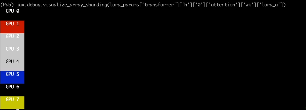
LoRA A Matrices (lora_a)

• The partitioning specification we used: PS("fsdp", "mp").

• Visualization:
  

  • Axis sharding: the sharding of lora_a parameters across axes will be (8, 1), meaning the first axis is sharded across 8 devices (axis fsdp), and the second axis is not sharded.

    

    The illustration shows that the first axis is sharded across 8 devices (axis fsdp), while the second axis is not sharded.

LoRA B Matrices (lora_b)

• Our partitioning specification used: PS("mp", "fsdp").

• Visualization:
  

  • Axis sharding: sharding of lora_b parameters by layers will be performed as (1, 8), that is, the second axis is sharded into 8 devices (axis fsdp), and the first axis is not sharded.

    

    The illustration shows that the second axis is sharded into 8 devices (axis fsdp), splitting the columns of the matrix.

This sharding strategy optimizes parameter distribution, reduces unnecessary communication overhead, and increases parallelism during training. It ensures that each device contains only a portion of the LoRA parameters, providing efficient scaling for large models like LLaMA 405B.

Updating only LoRA parameters

To optimize training when fine-tuning the LLaMA 405B model, we compute gradients only for the LoRA parameters, leaving the main model parameters frozen. This approach reduces memory usage and speeds up training because we update fewer parameters. Implementation details can be found in our GitHub repository.

In our training cycle, at each stage, a batch of input data is passed through the model. Since only the LoRA parameters are trained, the model predictions and the computed loss function depend only on these parameters. Then we perform backpropagation with the LoRA parameters. By focusing updates only on these parameters, we simplify the training process, allowing efficient fine-tuning of extremely large models like LLaMA 405B on multiple GPUs.

Conclusion

Fine-tuning the huge LLaMA 3.1 405B model on AMD GPUs using JAX left us with an extremely positive impression. Thanks to the powerful parallelism capabilities of JAX and its hardware-agnostic methods, I was able to efficiently distribute the model across 8 AMD MI300x GPUs. The use of parameter sharding allowed efficient management of the model's enormous parameter volume between devices, ensuring near-linear scalability and high memory efficiency.

This experience highlights the capabilities of AMD GPUs as a powerful alternative to NVIDIA hardware in large-scale AI training. The seamless integration of JAX with ROCm support simplifies the transition and opens up new opportunities for the AI research and development community. By sharing my experience and code, I hope to motivate others to explore and apply these tools in their own large-scale machine learning projects.