A brief guide to neural network quantization

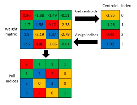
We literally reduce the bit depth of the data, which allows us to reduce computational resources and decrease the amount of memory needed to store models.

Our Nvidia card uses cheap, for example, 8-bit cores for performing convolution/matrix multiplication operations - we get a cheap model. Of course, such trimming of floating-point numbers can also lead to a decrease in accuracy. Catastrophic.

Different quantization methods have been invented, each of which has its own characteristics, approaches, and applications.

They are divided into three criteria: uniform and non-uniform quantization, symmetric and asymmetric quantization, as well as static and dynamic quantization. We will not go into detail. The main thing is that quantization can be done not only to 8-bit but also to 16-bit...

Where data with a high mass distribution from -1 to 1 is likely to fall within the range. The most important thing is that quantization is always an approximation, which can be costly. If you decide to reduce the memory size several times and literally convert float32 to int8, especially... That is, from floating-point to integer values.

If everything is bad, then, for example, static quantization is used. Otherwise, the model is immediately trained on "quantized" data.

Two Principles of Quantization

Practical implementation is carried out, for example, through Post-training quantization (PTQ) and is based on post-training transformation of the model, which has already completed training on data with high numerical precision, usually 32-bit floating point. This is the case when we expect our supermodel to survive such data reduction.

Therefore, the main goal of PTQ is to minimize memory and computational resource consumption during inference without the need to retrain the model.

In PTQ, model weights and, in some cases, activations are converted to lower precision integer values, most often 8-bit integers (int8), which significantly reduces the model size and speeds up computations by using SIMD (Single Instruction, Multiple Data) instructions at the hardware level.

SIMD operations process multiple data with a single instruction. This is their difference from traditional/scalar operations.

In PTQ, there are no changes in the neural network architecture, and the quantization algorithm is performed separately from the training process.

The main stages include quantizing floating-point weights to int8 by calculating scales and zero shifts, which allows preserving the value range. This is done using statistical information collected on a small amount of training data.

It is important that through PTQ, activations and weights can be quantized differently: activations can be dynamically quantized during inference depending on the input data, while weights are statically quantized based on a priori (initial) statistics.

If you are indeed working on a deep-deep neural network, there may be issues with accuracy, the same applies to tasks with high sensitivity in the data.

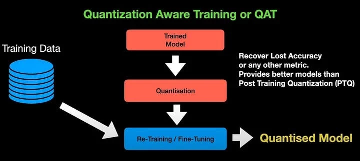
Quantization-Aware Training (QAT) is more complex - here quantization is taken into account already at the model training stage.

Unlike PTQ, in QAT the weights and activations of the model are represented in low-bit format (int8 or int16) throughout the entire training process, which allows the model to adapt to limited numerical precision.

The QAT architecture assumes that quantized versions of the weights are not used directly, but through emulation of the quantization process during the forward and backward pass of the model.

In the forward pass, weights and activations are modeled as quantized integers, which allows effective emulation of the inference process in a quantized environment. The backward pass, however, uses floating-point weights, which maintains the accuracy of gradient descent and allows the model to be adjusted under limited precision conditions.

During training, the model "learns" to compensate for errors caused by quantization, which reduces the accuracy losses observed with PTQ. QAT requires significantly more computational resources during training, as the training must take into account the quantization of all intermediate activations and weights.

At the same time, it is necessary to simulate quantization not only for the weights, but also for the input data at each layer, which increases the computational complexity of the model during training.

To implement QAT, it is necessary to modify the standard layers of the neural network in such a way that they support low-bit computations, as well as correctly configure the backpropagation mechanisms.

The use of QAT is often associated with tasks such as deployment on mobile devices, where computational resources and memory are limited. Therefore, such a quantization architecture is often used for CV tasks when we set up a camera with a microprocessor and expect a miracle of detection...

How does it work in practice?

In TensorFlow, quantization is implemented through TensorFlow Lite — a lightweight version of TensorFlow specifically designed for deploying models on resource-constrained devices, like a raspberry pi)))

PTQ in TensorFlow Lite can be performed using the post-training quantization method, where a floating-point trained model is automatically converted to a quantized version using the function converter.optimizations = [tf.lite.Optimize.DEFAULT].

This process includes static weight quantization using a small set of calibration data to calculate scales and zero-level shifts. An example of code in TensorFlow Lite for PTQ might look like this:

import tensorflow as tf

# Loading the model
model = tf.keras.models.load_model('model.h5')

# Converting the model using PTQ
converter = tf.lite.TFLiteConverter.from_keras_model(model)
converter.optimizations = [tf.lite.Optimize.DEFAULT]
tflite_model = converter.convert()

# Saving the quantized model
with open('model_quantized.tflite', 'wb') as f:
    f.write(tflite_model)

For a complex QAT scenario in TensorFlow, the built-in quantization functionality at the training stage is used, which allows considering the quantized representations of weights and activations during the training process.

Everything goes through tf.quantization.fake_quant_with_min_max_vars, where quantization is simulated in the forward and backward passes.

However, this requires more detailed network tuning and specific changes in the training process.

In PyTorch, quantization is supported through the torch.quantization package, which allows both post-training quantization and QAT.

In PyTorch, a modular approach allows coders to choose between symmetric and asymmetric quantization, as well as to implement both dynamic activation quantization and static weight quantization.

Before performing PTQ quantization in PyTorch, the model is prepared using the torch.quantization.prepare() function and converted using torch.quantization.convert().

An example of PTQ code in PyTorch:

import torch
import torch.quantization

# Loading the trained model
model = MyPretrainedModel()

# Preparing the model for quantization
model.eval()
model.qconfig = torch.quantization.get_default_qconfig('fbgemm')
torch.quantization.prepare(model, inplace=True)

# Applying PTQ
torch.quantization.convert(model, inplace=True)

# Testing the quantized model
output = model(input_data)

For QAT in PyTorch, a similar structure is used, but with the addition of a training procedure that takes quantization into account.

The model is first prepared through torch.quantization.prepare_qat(), and then training continues, during which quantization simulation occurs.

It is important to note that during training the model works with floating-point weights, but at the inference stage it is converted to int8.

ONNX (Open Neural Network Exchange) is an open format for representing deep learning models that ensures model portability between different frameworks.

For quantization in ONNX, onnxruntime is used, supporting both static and dynamic quantization.

Static quantization in ONNX works through calibration data - they are used to calculate quantized values before inference begins, while dynamic quantization is applied only to weights, simplifying the process and reducing the inference load.

An example of model quantization in ONNX might look like this:

import onnx from onnxruntime.quantization import quantize_dynamic, QuantType

model_fp32 = 'model.onnx' model_quant = 'model_quant.onnx'

Quantization with distillation and pruning

Often the quantization process is carried out together with other optimization methods - the same pruning or distillation.

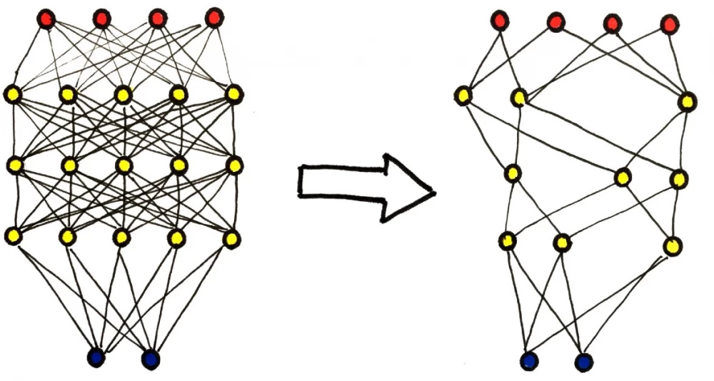
Pruning is a method in which unnecessary or inactive neurons and connections are removed from the network without significant damage to its performance.

Pruning can be performed based on various criteria, such as weights magnitude pruning, where weights with minimal values are removed, or sensitivity analysis pruning, where the contribution of each neuron to the overall model error is assessed.

In combination with quantization, pruning can significantly reduce the amount of computation, as only active neurons remain after pruning, on which quantization can be applied.

For example, after pruning, the model can be converted into a quantized version with fewer parameters, further reducing its computational complexity.

The practical implementation of pruning followed by quantization in TensorFlow might look like this:

import tensorflow_model_optimization as tfmot

model = tf.keras.models.load_model('model.h5')

prune_low_magnitude = tfmot.sparsity.keras.prune_low_magnitude
pruned_model = prune_low_magnitude(model)

pruned_model.compile(optimizer='adam', loss='sparse_categorical_crossentropy')
pruned_model.fit(train_data, train_labels, epochs=2)

converter = tf.lite.TFLiteConverter.from_keras_model(pruned_model)
converter.optimizations = [tf.lite.Optimize.DEFAULT]
tflite_quantized_model = converter.convert()

with open('model_pruned_quantized.tflite', 'wb') as f:
    f.write(tflite_quantized_model)

Step by step.

First, we load the model using tf.keras.models.load_model('model.h5').

This model can be a pre-trained neural network, for example, for image classification or speech recognition tasks.

The prune_low_magnitude method, which is part of the tensorflow_model_optimization library, is used to prune the model.

The method removes connections (neural weights) whose values are close to zero, thereby reducing the size of the model and the amount of computation it requires.

As a result, a pruned_model version of the model is created, in which some parameters are zeroed out. This helps to reduce the complexity of the model and speed up its execution without significant loss of accuracy.

After applying the pruning method, the model is compiled and fine-tuned on the training data using the fit() method. This is necessary for the model to adapt to the modified structure where some neural connections have been removed.

After the training is completed, the model undergoes post-training quantization using TFLiteConverter.

This process involves converting the model weights from 32-bit representation (FP32) to 8-bit integer (int8), which significantly reduces the memory footprint of the model and speeds up inference.

Optimizations specified through converter.optimizations = [tf.lite.Optimize.DEFAULT] are used in this process. After that, the model is saved in TFLite format, which allows it to be easily deployed on devices with limited computational resources, such as microcontrollers and mobile devices.

The principle of distillation is that the "large" model (teacher model) trains the "smaller" model (student model), transferring its knowledge in the form of predictions.

During the distillation process, the teacher model generates probability distributions of classes, which are then used to train the student model.

These distributions, also called "soft labels," contain more information than hard labels because they reflect the teacher model's confidence in each class.

Here is an example of distillation with quantization.

An example of the distillation process in PyTorch might look like this:

import torch
import torch.nn.functional as F
def distillation_loss(student_output, teacher_output, labels, T, alpha):
    soft_loss = F.kl_div(F.log_softmax(student_output / T, dim=1),
                         F.softmax(teacher_output / T, dim=1), reduction='batchmean') * (T * T)
    hard_loss = F.cross_entropy(student_output, labels)
    return soft_loss * alpha + hard_loss * (1. - alpha)
  for data, labels in train_loader:
    student_output = student_model(data)
    with torch.no_grad():
        teacher_output = teacher_model(data)
    loss = distillation_loss(student_output, teacher_output, labels, T=4.0, alpha=0.7)
    loss.backward()
    optimizer.step()

The distillation_loss function combines two components:

1. soft loss, which is calculated using the prediction distributions of the teacher model and the student model, normalized through temperature.

This helps to convey more detailed information about class probabilities to the student model, rather than just the correct class (hard labels), making the learning process more informative.

2. hard loss — a standard cross-entropy function that measures the distance between the student model's predictions and the actual class labels.

The combination of these two components (depending on the value of the parameter α) allows the student model to learn better based on the teacher model's predictions.

The student model training process:
In this code, the student model training loop looks as follows:

For each batch of data (mini-batch), inference is performed on both the student model and the teacher model.

The teacher model's predictions are fed into the loss function, where they are used to calculate the soft loss.

The loss function combines this with traditional cross-entropy (hard loss), training the student model more effectively.

Then the optimization step is performed, and the student model updates its weights based on the combined loss function obtained.

After training the student model using the distillation method, it can be quantized using standard methods such as dynamic or static quantization, which further reduces its size and resource consumption.

The integration of all three methods — quantization, pruning, and distillation — represents a powerful approach to model compression.

In real-world scenarios, such as mobile devices or embedded systems, this allows for significant improvements in model execution speed and energy efficiency.

For example, if the model is first pruned to remove insignificant connections, then undergoes the distillation process to create a lightweight version, and finally undergoes quantization, significant computational cost reductions can be achieved without losing critical accuracy.

This was a brief guide to quantization. We hope it was helpful for some, especially beginners.