Improving robot navigation using neural potential field

Introduction

For a mobile robot to move autonomously, it must be able to plan its movement trajectory. Often such planning is done in two stages.

In the first stage (global planning), it is necessary to connect the start and end of the required movement with a line so that this line does not touch obstacles. The line is most often broken, in planning terminology it is called a geometric path. A real robot usually cannot travel along a broken line; it has limitations on the turning radius of the wheels and, consequently, on the curvature of the trajectory.

Therefore, a second stage (local planning) is needed, in which the trajectory is smoothed or optimized. At this stage, the movement trajectory is determined taking into account all kinematic and dynamic constraints. Often, trajectory optimization is done as the robot moves: the robot moves along the geometric path and the nearest section of this path is optimized taking into account the most up-to-date obstacle data.

Such a concept of optimization in a sliding window mode in English literature is called Model predictive control. In Russian, this term is translated in different ways - "model-predictive control", "model predictive control", or even "control with predictive models". Our work is devoted to a specific issue: how to take into account the danger of collision with obstacles when optimizing a section of the trajectory?

For example, a penalty term responsible for avoiding collisions with obstacles can be added to the cost function of the optimization problem. If this term is considered as a separate mathematical function (it is called a repulsive or repulsive potential), it can be said that it forms an artificial potential field (Artificial Potential Field, APF).

The gradient of the potential field shows which way to shift the trajectory to make it safer. This allows the controller to find the right balance between the safety of the trajectory and its similarity to the reference path. In order to calculate the gradient, the repulsive potential function must be differentiable.

Calculating the APF values themselves is easy: for any point on the map, they depend on how far the nearest obstacle boundary is from the robot. But there is a problem with gradients: the distance to the nearest obstacle point is not a differentiable function, it is calculated algorithmically. It can be defined as such a function for some simple cases (for example, if the robot is round and there are few obstacles, and they are also round), but if we have a robot of complex shape moving on an arbitrary map, finding an analytical approximation of the APF becomes difficult.

Neural Potential Field

To deal with this difficulty, we proposed a model of the neural potential field (Neural Potential Field, NPField) — a neural network for calculating artificial potential. Our approach is conceptually inspired by the NeRF (Neural Radiance Field) model from the field of computer vision. NeRF takes as input the position and orientation of a virtual camera and returns the intensity of the image that such a camera could capture (which allows generating a view of the object from a new angle). Our model takes as input the position and orientation of the robot along with the obstacle map and returns the value of the repulsive potential. In practice, it is important for us not to obtain these values themselves, but to use their gradient for optimization.

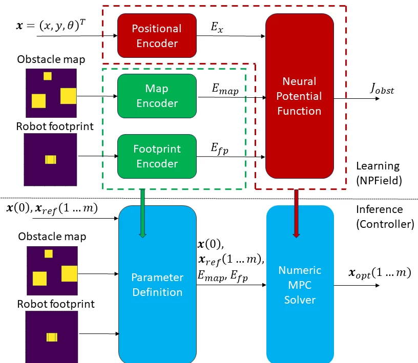
The general scheme of our approach is shown in the figure below:

At the top is the neural network diagram, at the bottom is the controller diagram used for trajectory planning. The neural network consists of two main parts: the encoder block and the neural potential function (NPFunction) - a subnetwork that computes the potential for a given robot position. In turn, the controller consists of two high-level blocks. The first block (Parameter definition) determines a set of parameters for the MPC task based on current data. This is done once per control cycle iteration. The second block (Numerical MPC Solver) performs the numerical solution of the optimization problem given this set of parameters.

NPField is trained as a single neural network and then split into two parts. Image encoders are included in the parameter definition block, and NPFunction is integrated into the numerical MPC solver. At each controller iteration, the encoders are called once, and the NPFunction is called and differentiated several times during the iterative optimization process.

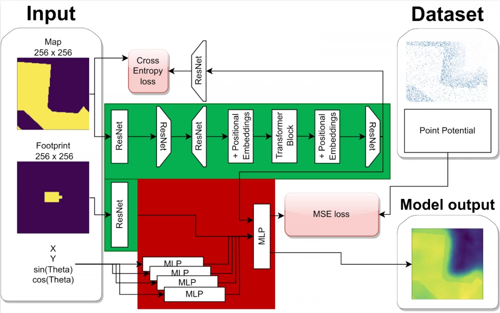
The neural network architecture is shown in more detail in the following figure:

Training Data

For training, we used data that includes the pose and shape of the robot, the reference value of the repulsive potential, and two-dimensional images of the obstacle map. The maps were taken from the MovingAI dataset. For each map, we generated a set of random robot positions and calculated their reference potential values using the following algorithm:

• The obstacle map is converted into a cost map:
  
  ◦ The signed distance function (SDF) is algorithmically calculated for each cell on the map. The SDF is the distance from the current cell to the nearest obstacle boundary. It is positive for free space cells and negative for obstacle cells.
  
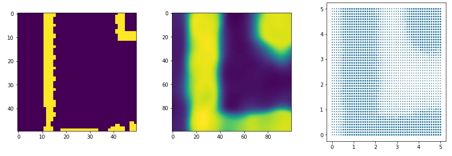
  ◦ The repulsive potential is calculated for each cell:

  

  Implementation and Experiments

  The numerical solution module MPC is implemented using the Acados framework, which relies on the lower-level CasADi framework. These frameworks allow for highly efficient solving of nonlinear optimization problems, with the developer's task reduced to correctly encoding the mathematical formulation of the problem. To integrate the neural network model NPFunction into the solver, we used the L4CasADi library.

Our local planner works together with the Theta* path planning algorithm, which generates a geometric path between the start point and the end point in the form of a broken line. It is worth noting that Theta* uses a simplified model of the robot's shape (a circle with a diameter equal to the width of the robot). This simplified model does not guarantee the safety of the path, which is ensured by our local planner.

We assume that obstacle maps have a resolution of 256×256, where each pixel corresponds to 2×2 centimeters of the real environment (i.e., the map size is 5.12×5.12 meters). For training, we collected a dataset based on MovingAI urban maps. It includes 4,000,000 samples taken from 200 maps for robots of two different shapes. Both robots correspond to the real mobile manipulator Husky UGV with the UR5 robotic arm. In the first case, the robot moves in space with the manipulator folded, in the second - with the manipulator extended. For each map with each robot, 10,000 random positions were generated. The dataset generation took 40 hours on an Intel Core i5-10400F processor.

One optimization procedure in our implementation takes 60-70 ms, of which parameter encoding takes about 10 ms, and the Acados solver takes the remaining 50-60 ms. It is worth noting that the Acados solver needs to be "warmed up" before use in real-time: the first execution of the optimization procedure may take about one second; after that, the solver works faster.

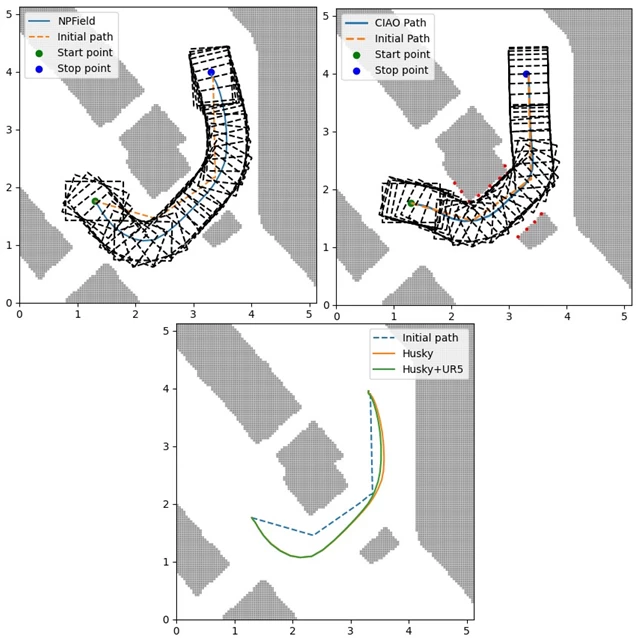
An example of a trajectory generated by our planner is shown in the upper left part of the figure below. The geometric path in the form of a line is transformed into a smooth and safe trajectory during optimization. Initially, the robot turns away from the obstacle and deviates from the global path, then smoothly returns to it, reaching the target position.

The lower part of the figure shows the difference between the optimization results for the robot with the folded and extended manipulator. The robot first drives to the flat wall, then turns and moves parallel to it. In this case, the robot with the extended arm turns slightly later than the robot with the folded arm. The yellow curve corresponds to the trajectory of the robot with the extended manipulator, and the green one with the folded one. The result shows that the model learns the different properties of the two footprints, which are useful for safer trajectory planning.

We compared the NPField trajectories with the baseline trajectory optimization algorithm CIAO, which is based on a convex approximation of the free space around the robot. The trajectory generated by CIAO is shown in the upper right part of the figure. It can be seen that the robot almost touches the edges of the obstacles. When tested on more diverse scenarios, CIAO failed to find a feasible path in almost half of the cases. This may be due to the fact that CIAO implements collision avoidance as a set of inequalities that are not differentiated during optimization. Therefore, it only checks for the fact of a collision, rather than trying to find a balance between safety and path deviation in the cost function.

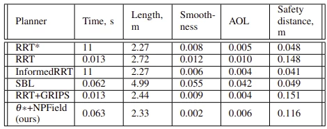
We compared our algorithm with the baselines on 20 scenarios using the BenchMR framework. The tasks include passing through narrow passages, similar to those shown in the figure above. We compared the standard metrics of the framework: planning time, path length, path smoothness (Smoothness), and Angle-over-length. All metrics are interpreted on the principle of "less is better".

The results are shown in the table below:

We compare our stack (Theta* + NPField) with popular planning algorithms: RRT, RRT*, Informed RRT, SBL, and RRT + GRIPS. In addition, the table does not include results for PRM, Theta* + CIAO, and Theta* + CHOMP, as these algorithms were able to find a path for less than half of the tasks. This result is especially important for Theta* + CIAO and Theta* + CHOMP, as they are optimization-based planners similar to our approach and use the same geometric paths. However, they were unable to handle the scenarios considered due to collisions (CHOMP) or inability to find a result (CIAO).

The results in the table show that our stack is generally comparable to other planners. It provides almost the shortest path length, the best smoothness, good AOL, good computation time, and good safe distance. We cannot point to an approach that is definitely better than ours (RRT with GRIPS is fast and safe but provides less smooth trajectories).

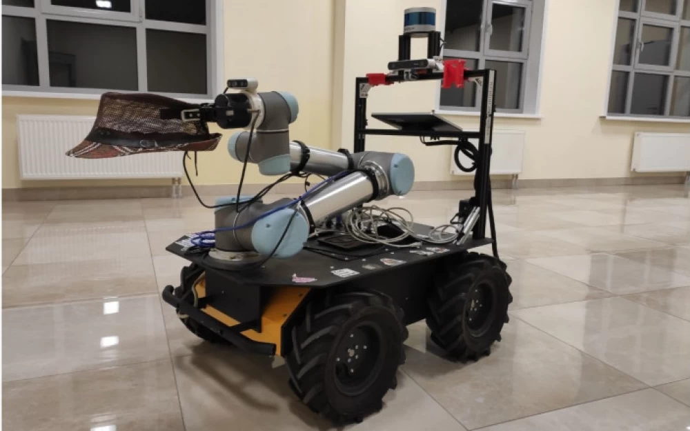
We deployed our approach on a real mobile manipulator Husky UGV as a ROS module for local planning and MPC control, which works with the global planner Theta*. The test scenario includes passing through a winding corridor. The manipulator holds the object in an unfolded state, so its shape is more elongated than usual. During our experiment, the robot successfully traversed a 15-meter path that included three turns and one narrow passage.

And below you can see how it travels along the route

Conclusion

We are very pleased with our result: it seems that neural potential is indeed capable of providing the best planning. However, this is just the beginning, as three turns and a narrow passage can hardly be called a difficult obstacle.

We are facing the complication of environments. First of all, this is the inclusion of elevation changes in the map - a new algorithm will be required to take them into account. The encoding of prints also needs development. This will be useful if the mobile operator controls the entire body and its print becomes variable.

I hope our experience was useful and interesting for you!