Topology in neural networks?

Often, when you hear about mathematics in ML, only Bayesian methods, derivatives, interpolations, and sometimes tensors are mentioned... But the mathematical apparatus in machine learning can go deep into the roots of even seemingly fundamental and abstract directions of this science.

Today we will touch a little on TDA, topological data analysis. We will try to write simply. So that even the most inexperienced student can understand. The goal of the article is to interest, because TDA is an avant-garde thing. But we need to start with the very basics: "Why and for what, and what is... this topology of yours?"

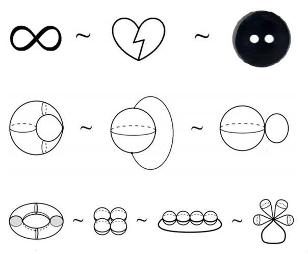
Topology deals with the study of properties of spaces that are preserved under continuous deformations. The first thing that comes to mind here is the theory of "gravity", the distortion of space-time... Unlike geometry, where sizes and shapes are important, topology focuses on properties that are resistant to changes without breaks and gluing.

To understand what this means, you can imagine a rubber sheet that can be bent, stretched, compressed, but cannot be torn or glued — the properties that are preserved under such changes are of interest to topologists. A classic example.

An important concept here is "continuity". If two objects can be transformed into each other through continuous deformations, they are called topologically equivalent. It's simple. A plasticine ball is equivalent to a plasticine cube.

A topological space is a fundamental concept in topology that extends the intuitive understanding of space. And this is the complexity of topology. It is a structure in which the concepts of "closeness" or "neighborhood" of points are defined, although this closeness may differ from the usual Euclidean geometry.

For example, on a sphere or a torus, the concept of neighborhood of points will differ from what we see in flat space. Moreover, in a topological space, one can talk about concepts such as open and closed sets.

Open sets are those in which each point is surrounded by other points of this set, while closed sets include their boundaries. The abstract level, of course...

The difficulty here is that it is hard for us to imagine a sphere as a space—we can only imagine a sphere in three-dimensional space. And this is the key difference and why this level of mathematics is rather in formulas. Which we will try to avoid.

Homotopy is a concept that describes the deformation of one object into another. Strictly speaking, two objects are homotopic if one can be continuously transformed into the other. Imagine we have a loop on a plane—if we can contract it to a single point without breaks and knots, then such a loop is homotopic to a point.

In more complex cases, such as on a torus (bagel), a loop that wraps around the hole can no longer be contracted to a point, and this is a fundamentally important difference between spaces with different topological structures. Homotopy helps us classify objects and spaces by their "deformability".

Homology is a more abstract way of studying topological spaces that connects algebra with topology. It allows us to study "holes" in spaces of different dimensions.

Homological groups are algebraic structures that describe the number and dimension of such holes.

For example, in a two-dimensional sphere, there are no holes either in the center or on the surface, while in a torus there is one "hole" in the center and one formed by the opening.

Thus, homology allows us to reduce topological problems to algebraic ones, making it possible to calculate topological invariants — characteristics that do not depend on the shape of the object.

With the development of computing technology, topology has found its place in data analysis. The application of topology to data is based on the fact that topological methods can reveal hidden structures in multidimensional or complex data sets, aka spaces, that traditional analytical methods may simply miss.

Topological Data Analysis

We will briefly go over the main principles and methodologies of data analysis, for now without coding nuances and tricks...

Topological data analysis (TDA) opposes traditional statistical and geometric approaches. It all comes down to identifying connected components, holes or voids, and their persistence as the scale or resolution of the data changes.

For example, persistent homology (i.e., the study of gaps when scaling spaces, our multidimensional data) is a fundamental method of TDA and serves to analyze topological invariants (manifold realizations) at different scales.

How do topological structures such as connected components, cycles, and voids change as the scale gradually increases? – this is the main question.

Of course, we are talking about computational topology, so we need tools to speak the language of discrete geometry, points, and segments...

Therefore, the verification is carried out through data filtration, where a sequence of simplicial complexes is created — abstract/discrete objects representing the connections between data points. This is conditional.

For example, several triangles can connect to form a polygon or even more complex shapes. We abstract the highlighted space or data set through understandable, separate, and countable objects that can be calculated.

If the question arises: "So the data is already discrete and countable, why translate anything?" – the answer is that topology is about working with sets without discretization.

Therefore, to reconcile data and topology, one needs to turn to computational topology, which allows working with these discrete data while remaining within topological logic.

At any given moment, a simplicial complex has certain topological characteristics, but as the scale changes, some structures appear while others disappear.

These "events" are recorded in so-called persistence diagrams, where the time of appearance and disappearance of topological invariants is plotted on the axis. Roughly speaking, we are simply tracking events, certain artifacts as we gradually increase the scale of our data.

The diagram visualizes the life cycle of each invariant, allowing us to distinguish significant (persistent) structures from noise (temporary).

Thus, persistent homology helps to identify the most stable topological characteristics of the data, which are preserved at different scales and, therefore, are the most informative.

Persistent diagrams can be visualized using barcodes — these are sets of segments, each of which denotes the time interval of existence of a particular topological structure.

Longer segments indicate more persistent and significant topological invariants, while shorter segments can be interpreted as noise fluctuations in the data.

Barcodes provide a visual representation of which topological structures dominate at various levels of resolution and help researchers gain a deeper understanding of the internal organization of the data.

Visualization of persistent diagrams through barcodes is a powerful tool because it allows for easy interpretation of complex multidimensional data structures by reducing them to simple and intuitive visual images.

But this is all cool, but how can we transparently and clearly and, of course, indirectly calculate

The closure theorem, which is also applied in TDA, describes an important topological characteristic of data related to the density and compactification of spaces.

In the context of data analysis, the theorem helps determine which parts of the data form closed sets and which remain open. This is important for understanding how structured the data is and how susceptible its topological shape is to changes.

The closure theorem plays a key role in identifying the boundaries of clusters and connectivity components, allowing for a more accurate interpretation of the topological properties of data sets.

The Mapper method is another significant TDA tool that serves to reduce the dimensionality of data while preserving the topological and geometric properties of the original space.

Mapper creates a simplified topological model of the data by breaking it into clusters and displaying them as a graph, where nodes represent clusters and edges represent connections between them. This method is useful for visualizing and understanding the structure of complex data sets because it allows you to see the relationships between different clusters, their internal connections, and holes.

Libraries for topological analysis

To calculate persistent homology or topological clustering, understandable algorithms are used. We have already indicated that simplicial complexes are needed to solve topology problems.

Simplicial complexes are built for different scales (levels of filtration), which allows data to be explored at different levels of detail. Next, homological groups are calculated for each scale, which helps to identify stable topological structures.

One of the popular algorithms is the Vietoris-Rips complex construction algorithm, which starts with the creation of simplices (groups of data points that can be considered as generalizations of triangles to higher dimensions) and continues through their filtration.

As the scale increases, simplices are added to the complex, and topological structures, connectivities, or cycles begin to appear.

The algorithm records the moments of appearance and disappearance of these structures, which are then interpreted through persistent diagrams.

This approach is widely used for data analysis in multidimensional conditions, as it is resistant to noise and can be adapted for high-dimensional data.

For example, GUDHI, Dionysus, and Ripser work with this algorithm, providing convenient tools for implementing these algorithms.

An example code using GUDHI might look like this:

import gudhi as gd

# Creating a simple simplicial complex
rips_complex = gd.RipsComplex(points=data_points, max_edge_length=2.0)
simplex_tree = rips_complex.create_simplex_tree(max_dimension=2)

# Computing persistent homology
simplex_tree.compute_persistence()

# Getting persistent barcodes
diag = simplex_tree.persistence()
gd.plot_persistence_barcode(diag)

Here we first create a simplicial complex based on the data_points, then compute its persistent homology and visualize the barcodes that show the life cycles of topological invariants at different levels of filtration.

Dionysus is another library that provides flexible tools for computing persistent homology.

Unlike GUDHI, Dionysus focuses on algorithms related to data filtration and simplicial complex management. It supports working with large data sets and multidimensional spaces, providing opportunities to customize algorithms for specific tasks.

Ripser is a specialized library for fast and efficient implementation of persistent homology computations. For mobile devices :)

To speed up computations in the context of large data sets, optimization methods such as reducing the size of simplicial complexes and using special data structures like KD-trees and grid methods are often applied.

For example, to avoid computing simplices for all possible combinations of points, sampling methods or approximate algorithms for data filtration can be used.

KD-trees allow efficient nearest neighbor searches, which is important for constructing Rips complexes.

This is especially relevant for high-dimensional data, where even small optimizations can significantly reduce computation time.

In addition, parallel computing and distributed systems are used, which allows processing very large data sets by breaking them into parts and performing computations in parallel.

For example, the Ripser library supports time and memory optimization by not storing all simplices in memory at the same time, which allows processing data sets that would not fit in memory using the usual approach.

Specific example of analysis

For example, we will use a data set of stock prices over a certain period. We will apply the method of persistent homology to identify stable topological structures in the data.

At the beginning of the program, the necessary libraries for working with financial data and their subsequent analysis are imported.

We load historical stock price data from a CSV file, using the pandas library for data processing.

We specify that the column with dates will be used as an index, and select only the column containing information about closing stock prices.

After that, the data is converted to monthly values using the resample function, which averages the values for each month. Missing data is removed using the dropna method to avoid errors in further analysis.

import pandas as pd
import numpy as np
import gudhi as gd
import matplotlib.pyplot as plt

# Loading stock price data
# For example, using Apple stock price data for the last 5 years
data = pd.read_csv('AAPL.csv', parse_dates=['Date'], index_col='Date')
data = data  # Using only the closing price column
data = data.resample('M').mean()  # Resampling data to monthly intervals
data.dropna(inplace=True)  # Removing missing values

Now we will bring the data to a format suitable for building simplicial complexes.

To do this, you can use the "shift" method to create a sequence of time windows. We will use fixed-length windows to form points in a multidimensional space.

The window size is set, for example, 12 months, and for each window, an array of closing stock prices is formed. This allows transforming time series into sets of points in a multidimensional space.

This approach is useful because topological analysis works with multidimensional data, and using windows allows extracting information about price dynamics in different periods.

# Defining the window length
window_size = 12  # 12 months
data_windows = []

for i in range(len(data) - window_size):
    window = data['Close'].iloc[i:i + window_size].values
    data_windows.append(window)

data_windows = np.array(data_windows)  # Converting to a NumPy array

In the next step, we use the GUDHI library to create a Rips complex based on the obtained points. The Rips complex is created using the RipsComplex function, which uses distances between points to build simplicial complexes.

The parameter max_edge_length sets the maximum distance between points at which they are considered connected, and the parameter max_dimension indicates that we will consider simplices up to the second dimension, i.e., segments, triangles, and other simple multidimensional structures.

# Creating a Rips complex
rips_complex = gd.RipsComplex(points=data_windows, max_edge_length=5.0)  # max_edge_length can be adjusted
simplex_tree = rips_complex.create_simplex_tree(max_dimension=2)  # Considering up to 2D simplices

Now we will compute the persistent homology for the resulting simplicial complex and visualize the results.

# Computing persistent homology
persistence = simplex_tree.persistence()

# Visualizing persistence diagrams
gd.plot_persistence_diagram(persistence)
plt.title("Persistent Diagram")
plt.show()

# Visualizing barcodes
gd.plot_persistence_barcode(persistence)
plt.title("Persistence Barcode")
plt.show()

After executing the above code, we obtain persistence diagrams and barcodes that visualize the persistent topological structures in the stock price data.

Persistence diagrams show which topological invariants were detected at different levels of filtration. Each segment in the barcode represents a time interval during which a particular topological structure existed.

If, for example, we see long segments in the barcode, this may indicate persistent trends or patterns in the stock price data.

If such patterns appear at different time scales, this may signal the presence of fundamental factors affecting price dynamics.

Through topological analysis, we can identify important structures such as stable price trends, cycles, and anomalies.

For example, if we observe that certain trends persist over a long period of time (as seen by long segments on a persistence diagram), this may indicate fundamental factors affecting the market, such as changes in supply or demand, economic events, or changes in the company.

Anomalies that may be represented by short segments may indicate market volatility or short-term price fluctuations caused by speculation.

Where else to apply topological analysis?

In bioinformatics, TDA helps analyze biological data, which usually has a complex and high-dimensional nature.

For example, protein structures, DNA, or transcriptomics data can be represented as multidimensional objects. Using persistent homology methods, one can study how the topological characteristics of these objects change as the filtration changes, which allows identifying stable structures such as loops or voids.

In genomics, topological analysis helps explore the relationships between genes, which may have a complex network nature, for example, genes responsible for certain biological processes may form stable topological structures.

In image analysis, topological analysis helps recognize complex shapes and patterns in the data.

Imagine an image as a set of points in a multidimensional space, each characterized not only by its coordinates but also by color, texture, and other features. TDA helps to highlight the main topological properties: object contours, their boundaries, as well as stable structures that persist when the scale or noise in the image changes.

Persistent homology allows us to evaluate how long certain patterns in the image exist when the filtration changes, which helps to improve image recognition or object classification algorithms.

For example, in medical diagnostics, TDA helps to accurately delineate boundaries between different types of tissues or pathological formations.

Financial data also has a complex multidimensional nature. Stock prices, exchange rates, trading volumes—all these are time series that can be analyzed using topological methods.

Using TDA, hidden trends, cycles, or anomalies in price dynamics can be identified, which may go unnoticed when using traditional methods.

Topological analysis, for example, allows us to identify stable price patterns that may indicate long-term market trends, as well as anomalous structures that may indicate volatility or sudden price changes.

Persistent homology helps to analyze how these patterns change depending on the time scale, which can be useful in developing trading strategies or risk management.

And where would we be without research?

Neural networks have a complex topological structure, especially in the context of deep learning, where the model can contain many hidden layers and parameters.

Using TDA methods, one can study the topological properties of data passing through the network, analyze how neural activations form complex structures at various levels of abstraction.

For example, in image classification tasks, persistent homology can be used to analyze the output layers of a neural network to understand how the network interprets input data, as well as identify errors or gaps in the model's generalization...

Additional literature for the most curious

• “Topological Data Analysis for Machine Learning: A Survey”

  • Link to the article

• “Topological Deep Learning: A Review of an Emerging Paradigm”

  • Link to the article​(SpringerLink)

• “Explaining the Power of Topological Data Analysis in Graph Machine Learning”
  The article explores the role of TDA in graph analysis, demonstrating how alpha complexes and filtrations can improve the understanding of the shape and connectivity of data in graph structures. This is useful for analyzing social networks and protein interaction networks.

  • Link to the article​(ar5iv)

• “A Topological Machine Learning Pipeline for Classifying Disease Subtypes”
  The article shows how topological data analysis can be applied in bioinformatics to classify disease subtypes by examining the persistence of topological features in biological data.

  • Link to the article