Hypernetworks: Neural Networks for Hierarchical Data Processing

The work of neural networks is inseparable from the assumption that a single function maps inputs to outputs. However, in real-world conditions, data rarely fits such frameworks.

Suppose there is a clinical study being conducted across several hospitals. The drug is the same, but the patient populations, procedures, and recording methods differ. In such cases, the observations are grouped into different datasets, each governed by hidden parameters.

Standard neural networks fail rigidly under such conditions. Train a single model on all datasets at once — and it will lose focus due to the differences, averaging functions that should not be averaged. Train separate models on each dataset — and you will get overfitting, especially if the datasets are small. Workarounds such as using static vector representations (embeddings) or constantly increasing the size of the network do not fundamentally solve the key problem: the system memorizes quirks of the network without modeling its structure, which forms at the dataset level. And it is this structure that is the key to quality results.

In this post, we will analyze an alternative approach, namely the creation of hypernetworks. With their help, we can teach neural networks to adapt to the dataset. A hypernetwork will not memorize a single fixed mapping but will learn to generate parameters for another network based on the dataset obtained as an embedding. As a result, the model will be able to:

• Infer properties affecting the entire dataset level based on just a couple of data points,

• Adapt to entirely new datasets without retraining, and

• Accumulate information taken from different datasets to enhance stability and mitigate overfitting.

In this article, we will build a model step by step. Accompanying it is code that you can run and test on synthetic data generated based on Planck's law. As we study this topic, we will also compare hypernetworks with traditional neural networks and uncover the mystery of why, in some cases, Bayesian models can perform even better.

1. Introduction

When solving many realistic problems, it is necessary to work with data that is hierarchical by nature: observation results are grouped into interrelated but different datasets, each governed by its inherent hidden properties. For example, consider a clinical trial testing a new drug. The study involves multiple hospitals, and during the work, it is recorded what dosage each patient received, along with data on how it affected the patient. Naturally, the main factor determining the outcomes of the study is the effectiveness of the drug. However, certain conditions specific to each hospital also play a role. Demographic data about patients, procedural differences, and even the method of recording results can also lead to adjustments in the final outcome. If these differences are significant, then the data cannot be interpreted as coming from just one population, as this would lead to incorrect conclusions about the drug's effectiveness.

From a machine learning perspective, the configuration is quite complicated. The properties operating at the dataset level—namely, how results vary from hospital to hospital—are implicit: they exist but are not directly observed. A standard neural network will learn exactly one fixed correspondence between some input and some output data, but this correspondence is ambiguous here. Two different hospitals, where implicit conditions differ, will yield different results even for patients with identical profiles. The function becomes well-defined (that is, unambiguous) only when it accounts for factors operating at the level of individual datasets.

To specify these statements, let's construct a simplified example in which we will try to quantitatively express the indicators of interest in our research. Each dataset will consist of observations (𝝂, y), derived from a simple hierarchically structured function. We will generate the function according to the Planck law:

where:

• 𝝂 is the covariate (frequency),

• y is the response (brightness or flux),

• T is a parameter specific to the dataset (temperature). Within this dataset, this parameter is constant, but it can vary from dataset to dataset; finally

• ε is Gaussian noise with a scale factor σ, which remains unknown but is the same across all datasets.

Based on this data, it would be possible to map pixels on an image visualizing temperature. Each pixel in the image "has" its own surface temperature T, from which its spectrum depends, while the scale of the noise σ is a property of the spectrograph or amplifier that remains consistent across the entire range of observations.

In this case, the most important thing is that, while the modeling person observes and knows the pairs (𝝂, y), the parameter T is part of the function generating the data and is unknown to the observer. While the function f(𝝂; T) is constant (each dataset fits into the same general equation), each dataset has its own particular T, so the mapping of y(𝝂) varies from dataset to dataset. This fundamental structure—containing dataset-specific hidden variables that influence the observed correspondences—can be found in realistic problems everywhere.

If we approach the problem straightforwardly and train a single model on all datasets at once, we will force the network to ignore these latent differences and approximate the "average" function. This approach is fundamentally unsuitable for working with heterogeneous data. Adapting the model for each dataset is also not a solution. If the dataset is small, there simply aren't enough data points for the model to learn confidently. Moreover, the shared functional structure along with shared parameters, such as the noise scaling factor σ, cannot be reliably estimated without resorting to pooling information.

On the contrary, it is precisely for such cases that we need a hierarchical model—one that simultaneously accounts for variability specific to individual datasets while also establishing information exchange between datasets. When using neural networks, this path logically leads us to meta-learning: models that not only learn the function but also learn how to properly learn functions.

Conclusion

The operation of standard neural networks is based on the assumption that one function can encompass all data. However, (very common) hierarchical data fundamentally do not conform to this assumption. We need models that can adapt to each dataset when necessary, while still sharing information that is consistent across different datasets.

2. Why Standard Neural Networks Struggle with Hierarchical Data

A standard neural network trained directly on pairs (𝝂, y), in the configuration described above, fails due to the assumption that there exists one universal function capable of relating input values to output values across all datasets at once. However, in the problem we have formulated, each dataset adheres to its own function y(𝝂), which depends on a hidden parameter T specific to that particular dataset. We do not have a unique function f(𝝂; T) because we cannot observe the parameter T. Without explicit access to T, the neural network cannot know which particular mapping to use.

Ambiguous Mappings

To make it clearer what the problem is here, let’s try to predict a person’s height without relying on any additional information. In a homogeneous population — say, where only adults are present — the typical average will be a good enough prediction. For example, if the population in question is adult Dutch women, then the average value in 68% of cases will correspond to the actual height of a woman within an error margin of ± 5 centimeters. But let’s assume that the dataset includes both adults and children. If there is only one distribution, the model will inevitably learn the “average” height, which will not be adequate for either children or adults. Predictions using the average in this way are almost never correct.

A similar problem arises in our hierarchical situation: since there is no single function that covers all datasets, predictions based on the “average” function will not be very accurate.

Common workaround strategies and why they are insufficient

• Static embeddings in the dataset: often, an attempt is made to assign a unique vector representation (embedding) to each dataset, extracted from a lookup table. This allows the network to remember which adjustments correspond to each specific dataset. However, this strategy does not generalize: a new dataset arrives, and the network has no vector representation for it, so it cannot adapt to work with the new dataset.

• Shortcut learning: another option is to simply increase the network and fill it with additional data. In principle, the model can capture subtle statistical cues—differences in noise patterns or input distributions—that indirectly encode the dataset index. But such "shortcut learning" turns out to be both inefficient and unreliable. The network memorizes quirks specific to individual datasets instead of doing what is needed—that is, it does not explicitly model the differences that arise at the dataset level. In applied fields, this leads to a shift: for example, the network may learn to incorrectly use a proxy variable (such as a postal code or demographic data), resulting in unfair or unstable predictions.

What we really need

These shortcomings help to understand what requirements for hierarchical data models are truly relevant. We do not force a single network to simultaneously approximate each of the datasets; we just need a model that can:

• Infer properties applicable to the entire dataset based on a few examples,

• Adapt to completely new datasets without retraining from scratch, and

• Effectively accumulate data from different datasets so that the shared structure (for example, functional form or noise scaling factor σ) is assessed more reliably.

Standard neural networks with a fixed structure simply cannot meet these requirements. To move forward, we need a model that dynamically adapts to the specific structure of the dataset while continuing to learn from data drawn from different datasets. Hypernetworks are an interesting attempt to approach this problem.

Conclusion

Such tricks as the use of static vector representations or model aggregation do not solve the key problem: due to factors hidden in the dataset, the mappings from input data to output become ambiguous. A neural network, the function of which by definition results in a single value, cannot encompass such data. A model is required that (1) outputs properties directly from the entire dataset, (2) adapts to new datasets, and (3) accumulates knowledge drawn from different datasets.

3. Neural Networks Adapt to the Dataset

3.1 Vector Representations of Datasets

When creating a network that adapts to the dataset, the first step is to provide the model with a way to represent variability at the dataset level. To this end, we will introduce the vector representation of the dataset: a latent vector E that summarizes the properties of the dataset as a whole.

We will assign an accessible learning representation to each training dataset:

# vector representations of the dataset (initialized with random values and updated during training)
dataset_embeddings = tf.Variable(
    tf.random.normal([num_datasets, embed_dim]),
    trainable=True
)

# Assigning dataset indices to each sample
dataset_indices = np.hstack([np.repeat(i, len(v)) for i, v in enumerate(vs)])
x_train = np.hstack(vs).reshape((-1, 1))
y_train = np.hstack(ys).reshape((-1, 1))

# Extracting dataset-specific vector representations 
E_train = tf.gather(dataset_embeddings, dataset_indices)

At first glance, the code may remind one of regular searching through vector representations. In such a situation, each dataset is assigned a static vector extracted from a table—but we have already discussed in detail why this approach will not work in this case!

During training, these vector representations indeed function as standard vector representations (and are implemented that way). Our vector representations, like the standard ones, are needed to encode properties specific to the dataset. The key difference here lies in how exactly we handle the vector representations at the logical inference stage: learning can continue on the vector representations, even during prediction. If a dataset that the model has not seen before arrives during logical inference, we initialize new vector representations for this dataset and optimize it on the fly. As a result, the vector representation becomes a function of the dataset itself rather than a hard-coded (and therefore constant) identifier. During training, the model learns the vector representations that capture the factors hidden in the data generation process (for example, concerning our task — the parameter T). The vector representation continues to adapt during the prediction stage, allowing the model to represent new datasets that it has not seen before. This flexibility is critically important for generalizing data.

3.2 Introduction to Hypernetwork

When the vector representations of the datasets are ready, we need a mechanism that allows us to translate these vector representations into meaningful changes in the behavior of the network. The most natural way to do this is through a hypernetwork: a secondary neural network that generates parameters for the main network.

This is both a simple and powerful idea. We study not a single function f(𝝂), but a family of functions f(𝝂; E), parameterized by the vector representation of the dataset E. The hypernetwork takes E as input and produces weights and biases for the first layer of the main network. In this case, the way the main network processes the incoming data directly depends on the dataset-specific information. The rest of the network, except for the first layer, operates independently of the dataset. In fact, we have factored the family of functions f(𝝂; E) into the composition g(𝝂; h(E)), and our task is to learn the functions g and h that approximate our data generation process.

Here is a minimal implementation using Keras:

def build_hypernetwork(embed_dim):
    """Generate parameters for the first layer of the main network"""

    emb = K.Input(shape=(embed_dim,), name='dataset_embedding_input')

    l = K.layers.Dense(16, activation='mish', name='Hyper_L1')(emb)
    l = K.layers.Dense(32, activation='mish', name='Hyper_L2')(l)

    # Generate weights for the layer (32 hidden units, 1 input feature)
    W = K.layers.Dense(32, activation=None, name='Hyper_W')(l)
    W = K.layers.Reshape((32, 1))(W)  # Reshape to (32, 1)

    # Generate biases (32 hidden units)
    b = K.layers.Dense(32, activation=None, name='Hyper_b')(l)

    return K.Model(inputs=emb, outputs=[W, b], name="HyperNetwork")

The hypernetwork transforms the vector representation of the dataset into a set of layer parameters (W, b). These parameters will replace the fixed weights present in the first layer of the main network, resulting in the input data being transformed according to the specifics of the dataset, and learning can occur on the resulting output.

The hypernetwork maps vector representations of datasets to neural network parameters. This directly captures the variability present at the dataset level, so that each dataset is modeled with its own effective function, eliminating the need to train separate networks from scratch. Notably, despite all this flexibility, all parameters of the hypernetwork remain constant relative to the dataset. The dataset-specific information we need to achieve this flexibility is just one vector representation (in our case — 4 floating-point numbers per dataset).

3.3 Integration with the main network

So now we have a hypernetwork to generate dataset-specific parameters, and the next step is to integrate these parameters into the main network modeling the data. The main network can have any architecture we desire; all that needs to be done is to replace the first fixed linear transformation with a dataset-specific transformation derived from the vector representation.

To do this, a custom layer can be defined that will apply the weights and biases generated by the hypernetwork:

class DatasetSpecificLayer(K.layers.Layer):

    def __init__(self, **kwargs):
        super(DatasetSpecificLayer, self).__init__(**kwargs)

    def call(self, inputs):
        """ Applies a transformation specific to the dataset using the generated weights """

        x, W, b = inputs  # unpack inputs

        x = tf.expand_dims(x, axis=-1)       # Shape: (batch_size, 1, 1)
        W = tf.transpose(W, perm=[0, 2, 1])  # Transposing W to (batch_size, 1, 32)

        out = tf.matmul(x, W)          # Shape: (batch_size, 1, 32)
        out = tf.squeeze(out, axis=1)  # Shape: (batch_size, 32)

        return out + b  # Adding bias, final shape: (batch_size, 32)

This layer serves as a bridge between the hypernetwork and the main network. We do not rely on a single fixed set of weights; instead, the transformation applied to each input sample is tailored to the dataset through its vector representation.

With this component set up, we can define the main network:

embed_dim = 4
hypernet = build_hypernetwork(embed_dim)

def build_base_network(hypernet, embed_dim):
    """ The main network that takes x and the dataset's vector representation as input """

    inp_x = K.Input(shape=(1,), name='input_x')
    inp_E = K.Input(shape=(embed_dim,), name='dataset_embedding')

    # Obtain dataset-specific weights and biases from the hypernetwork 
    W, b = hypernet(inp_E)

    # Based on the generated weights, obtain the custom layer 
    l = DatasetSpecificLayer(name='DatasetSpecific')([inp_x, W, b])

    # Continue working with a normal dense network 
    l = K.layers.Activation(K.activations.mish, name='L1')(l)
    l = K.layers.Dense(32, activation='mish', name='L2')(l)
    l = K.layers.Dense(32, activation='mish', name='L3')(l)
    out = K.layers.Dense(1, activation='exponential', name='output')(l)

    return K.Model(inputs=[inp_x, inp_E], outputs=out, name="BaseNetwork")

Why is exponential activation used in the last layer? The results of the calculations based on Planck's law are strictly positive, and large x corresponds to exp(-x). Therefore, this choice reflects our anticipated solution and encourages a roughly linear output from the Mish activation in layer L3 to naturally transform into an exponential tail. We arrived at this variant based on the physics of the dataset and found that this option provides faster convergence of the model and better generalization. Exponential activations can lead to convergence issues for large values along the y-axis, but there are no such values in our dataset.

Let me remind you how the entire process is structured:

• Hypernetwork generates parameters (W, b) specific to this dataset.

• Then, DatasetSpecificLayer applies this transformation to the input value 𝝂, resulting in a transformed representation 𝝂'. If the transformation works correctly, all different datasets should be directly comparable to each other in the transformed space.

• Main network learns one universal mapping from transformed inputs 𝝂' to outputs y.

By integrating the parameters generated by the hypernetwork into the first layer, we transform the main network into a system that automatically adapts to each dataset. This allows us to capture the structure specific to each dataset while continuing to train one model on all datasets.

Conclusion

By combining vector representations of datasets with the hypernetwork, we can express an entire family of functions f(𝝂; E) using a neural network based on a bijective function. To do this, it needs to be decomposed into f(𝝂; E) = g(𝝂, h(E)), where g and h are standard bijective neural networks. The first layer of the main network acquires the specificity of the particular dataset, while the rest of the neural network continues to operate like a regular feedforward network and learns a universal mapping to the transformed input values.

4. Training Results

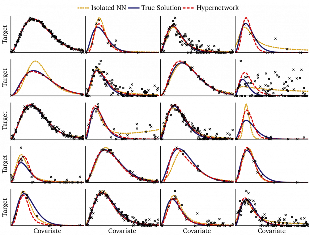
Now, having stitched together the vector representations, the base network, and the hypernetwork, we can test our model by checking it on a test task. For this, we will train it on a collection of 20 synthetic datasets obtained according to Planck's law as described in section 1. Each dataset has its own temperature, denoted as parameter T, while one common scale factor of noise σ is jointly used by all datasets.

The next figure shows the training results. In each of the sections, one of the datasets used during testing is presented. Each section contains:

• Solid blue line, corresponding to the true function derived from Planck's law,

• Black dots — these are the observed training data,

• Red dashed curve — these are the predictions made based on a model that relies on a hypernetwork and

• The curve of golden dots — these are the predictions generated by a regular neural network trained separately on each dataset.

Several patterns immediately stand out:

• Comparable Overall Accuracy: often (for example, in the 1^st column of the 1^st row) the predictions of the hypernetwork (in red) are very similar to the predictions of the isolated neural network (in gold). Therefore, despite the fact that we strictly limited the model and removed ~95% of its parameters, when using parameters across all datasets, even with a clear data deficit, the accuracy of the datasets is not compromised.

• Increased Stability: when the training data is sparse (for example, as in the 1^st column of the 2^nd row or in the last column of the 3^rd row), the hypernetwork overfits significantly less than the isolated neural network. Its predictions remain smoother and closer to the true shape of the function, while the isolated neural network sometimes fails to fit into discrete points.

• Accumulation of Data from Different Datasets: by training on all datasets simultaneously, the hypernetwork learns to separate the shared structure [for example, the noise scale factor σ or the underlying shape of the function f(𝝂; T)] from dataset-specific variations (the vector representation E). This shared learning stabilizes predictions across their entire spectrum, but is particularly evident in sections where the data is heavily noisy (as in cases with the last column of the 2^nd row or the 2^nd column of the 3^rd row).

Conclusion

With an abundance of data, the hypernetwork achieves accuracy comparable to that of isolated networks, while when data is scarce, it performs much more accurately than isolated networks. This advantage is achieved through the accumulation of information from different datasets, allowing the network to capture both general and dataset-specific structures within a single model.

5. Prediction for New Datasets

It is inspiring to see how well our hypernetwork learns. But the real test for it lies in how successfully it can adapt to new datasets that it has never seen before. Unlike a traditional neural network, which simply applies learned weights to any new input, our model is structurally designed to recognize that each dataset follows its own specific function. To make predictions, it must first logically derive a vector representation of the dataset.

5.1 Two-step process

Adapting to a new dataset occurs in two stages:

• Optimizing the vector representation of the dataset E' so that this representation explains the observed points.

• Using the optimized vector representation E' to generate predictions for new input data through the main network.

With such a two-step pipeline, the model, relying on a few observations, can capture properties specific to the particular dataset. There is no need to retrain the entire network.

5.2 Optimizing the vector representation

To logically derive the vector representation of the dataset, we consider E’ as a learnable parameter. We will not train all the weights of the neural network from scratch; instead, we will optimize only the vector representation of the dataset until the neural network adapts to it. Since the dimensionality of this vector representation is low (in this case, just 4 floating-point numbers), such optimization is effective, and only a small amount of data is required for convergence.

It is convenient to implement this using a wrapper model, which contains just one vector representation, which is then set as a variable that can be learned:

class DatasetEmbeddingModel(K.Model):

   def __init__(self, base_net, embed_dim):
       super(DatasetEmbeddingModel, self).__init__()
       self.base_net = base_net
       self.E_new = tf.Variable(
           tf.random.normal([1, embed_dim]), trainable=True, dtype=tf.float32
       )
       # for higher performance on relatively small datasets, use tensorflow_probability:
       # self.E_new = tfp.distributions.Normal(loc=0, scale=1).sample((1, embed_dim))


   def call(self, x):
       # Tile E_new across the batch dimension so that x matches the batch size 
       E_tiled = tf.tile(self.E_new, (tf.shape(x)[0], 1))
       return self.base_net([x, E_tiled])

   def loss(self, y_true, y_pred):
       mse_loss = K.losses.MSE(y_true, y_pred)
       reg_loss = 0.05 * tf.reduce_mean(tf.square(self.E_new))  # L2 regularization on E
       return mse_loss + reg_loss

Here, the vector representation of the dataset E’ is initialized randomly and then updated using gradient descent to minimize the prediction error on observed points. Since we are optimizing only a handful of parameters, this process is lightweight and well-suited for working with small datasets.

By framing the vector representation as a learnable parameter, the model can effectively adapt to new datasets. With this strategy, there is no need to retrain the entire network, while still capturing variations specific to the particular dataset. All of this is necessary for accurate predictions.

5.3 Generalization

One of the most outstanding advantages of this approach is the ability to generalize data from completely new datasets based on minimal data. In practice, models often require only ten data points to adapt. This few-shot adaptation is feasible because the hypernetwork has already learned the structured mapping from the vector representation of the dataset to the function parameters. When a new dataset arrives, it is sufficient to learn its vector representation without fine-tuning all the weights of the network.

Compared to traditional neural networks, which require hundreds or thousands of examples for effective fine-tuning, such adaptation based on vector representations allows for much more efficient use of data. With this approach, the model handles realistic scenarios in cases where it is impractical to collect large amounts of data for each new dataset.

5.4 Limitations

Despite these strengths, the hypernetwork approach is not perfect. When interpreting predictions made on out-of-sample datasets—those generated by the same method as the training data but not included in the training set—the quality noticeably degrades, especially with noisy or censored data, as well as very small datasets. This is illustrated in the following examples:

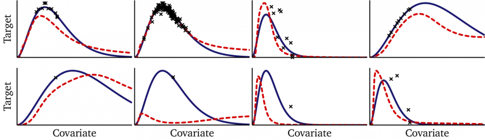
On the other hand, this is expected: it is exceptionally challenging to work with out-of-sample datasets, and no machine learning model can guarantee perfect generalization on previously unseen data. However, considering the performance it displayed on the training set, the results obtained on real material are somewhat disappointing. While adaptation to a specific dataset is indeed possible, the forms of functions learned by the hypernetwork are not always maintained once it encounters data that were not included in the training phase.

To summarize the data, a hypernetwork requires only a few examples, as we are not training the network anew but merely adapting the vector representations to new data. However, the performance of such networks significantly drops on data that was not present in the sample, so to increase reliability, we may need alternative approaches.

The degradation observed in this case somewhat resembles overfitting. It may be caused by the optimization stage we ran during logical inference, and with some other combination of step size, stopping criteria, regularization, etc., the results might have been better. But we were unable to find such a combination. On the contrary, it can be assumed that this degradation is fundamentally due to maximum likelihood estimation (which in terms of neural networks is optimization). Optimization is problematic not only because it is conducted at the logical inference stage but also as a learning algorithm in principle.

Conclusion

When working with new datasets, we optimize only a small vector representation E’ (on a few examples), rather than fine-tuning the entire network. The hypernetwork adapts quickly but may not operate very stably (compared to the results obtained on the training sample) on data whose examples were not considered during training.

6. Discussion and Next Steps

The hypernetwork approach demonstrates how neural networks can work not only through brute memorization but develop towards structured adaptation. By utilizing the vector representations of datasets and transforming them through the hypernetwork into model parameters, we were able to design a network capable of logically establishing the structure of each specific dataset, rather than simply averaging the function across all datasets. Because of this, the model can make generalizations based on limited data — this expresses the intelligence of the system.

The results we obtained highlight both the strengths and weaknesses of this strategy:

Strengths

• For adaptation, just a few examples are enough: the model adapts well to new datasets, and for this, it requires only a minimal set of observations.

• Collaborative learning: by accumulating information from different datasets, the stability of the system increases and overfitting is mitigated.

• Flexible architecture: using the same technique, the hypernetwork framework can be expanded into increasingly rich hierarchical structures.

Weaknesses

• Decreased performance when working with data that did not make it into the training sample: predictions become unstable on material from small, censored, or noisy datasets.

• Implicit structure: vector representations capture the differences between datasets, but without explicitly defined prior inputs, the model simply cannot incorporate explicit data, and it also struggles to maintain uniform function forms.

All these trade-offs indicate that hypernetworks are a promising but not perfect technology. They can be improved. For example, they lack explicit probabilistic structure, which is necessary for reasoning about uncertainty and for limiting extrapolations. This motivates us to touch on another family of models: Bayesian hierarchical networks.

With Bayesian approaches, we process hierarchical data directly, modeling dataset-specific parameters as latent variables drawn from existing distributions. When you work with uncertainty so explicitly, more stable predictions result, especially when dealing with small datasets whose data were absent from the training sample.

The next figure shows predictions made by Bayesian models on the same "out-of-sample" datasets that we tested earlier:

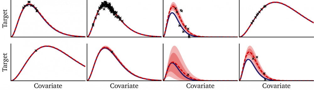
When comparing these predictions made on out-of-sample data with those made by the hypernetwork, the results of the Bayesian model may seem almost magical!

Hypernetworks introduce an element of meta-learning into hierarchical modeling, thereby ensuring flexible and efficient adaptation to the available data. But when it comes to reliability—especially regarding examples that were absent from the training set—Bayesian models seem clearly more advantageous. Together, these models complement each other and demonstrate how to adapt machine learning to work with hierarchical data.

Conclusion

Hypernetworks adapt well to the structure of the dataset, and they require only a few examples for training. However, they suffer from a lack of explicit prior information and from uncalibrated uncertainty.