Neural Query Optimizers in Relational Databases: On the Way to Productionization

Introduction

In the previous article, we talked about the pioneers in the field of neural network optimizers who created a foothold for the development of such ML systems and their subsequent introduction to the level of commercial products. In this one, we will touch on relatively stable approaches that do not require giant computing clusters and satisfy most business needs. Of course, there is no silver bullet, but with each of these methods, you can come to an optimal solution for a specific task.

Bao

Bao can be seen as a logical continuation and development of the ideas laid down in Neo. Moreover, the creators of Bao and Neo are the same people!

This model, although it appeared 4 years ago, is still featured in comparisons, and a large number of modifications are made based on it. Bao took on the task of correcting the shortcomings that prevented the industry from implementing neural optimizers in product solutions. For example:

1. The need for a large amount of data to train the model. Firstly, they may not be available in practice, and secondly, some models need to be trained for several days before reaching the level of basic optimizers.

2. Lack of quick adaptation of the model to a new DB schema, change in workload when executing queries, change in data volume, etc. That is, even after training the model to work well in a specific context, the slightest change in the environment negates all the benefits obtained from the neuro-optimizer — everything will have to be done anew.

3. Difficulty in debugging and interpreting results. The vast majority of neural network approaches are monolithic black boxes, the interpretation and debugging of which are extremely difficult.

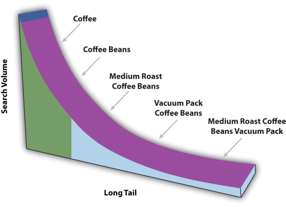
4. Very poor performance on a small number of queries (the so-called tail example problem). The fact is that on average the trained neuro-optimizer generates a plan of higher quality than standard optimizers. If you take the most typical query, it will work well. However, on rare, unique queries, the quality of the neural network can drop significantly (up to 100 times) — this is simply unacceptable in most real-world tasks. What if important system logic is built on such a query? There is a good illustration to understand the concept of the tail in our example:

Thus, for "Coffe" and "Coffe Beans" everything will be fine, because they create the main backbone of training examples (in the distribution trampoline scheme it starts with them, so their number will be overwhelming). But for an example like "Medium Roast Coffee Beans Vacuum Pack" it will be a disaster. This example almost does not fit into the general canvas, and there are not so many of them - so the model will simply prefer to ignore the error that occurs when processing such tail elements, even if it is colossal.

To surpass both open-source and commercial optimizers, training Bao (Bandit optimizer) can take up to several hours. With all this, it will not allow strong errors on tail queries, as previous approaches did. Also, Bao continues to perform well when the DB schema, workload, and table data change. It does not cancel all the previous developments of manually tuned optimizers - as much as we would like to admit, they contain the wisdom of several generations of the smartest programmers. So why not use it together with our learning machines?

Algorithm Analysis

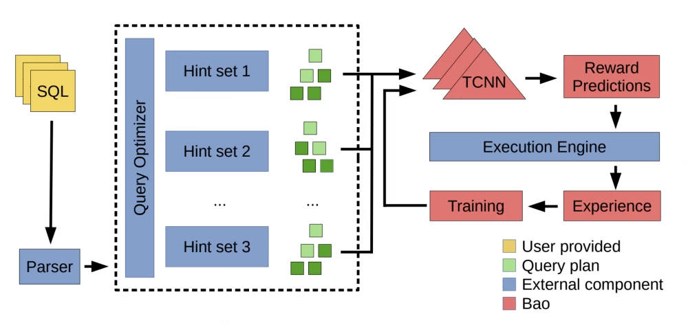
The main idea of Bao is to stand above the basic optimizer and give it rough hints, focusing on the current query and whether there is any information in the cache. For example, the model will decide that it is better not to apply loop joins in a certain situation or to refuse sequential table scans in favor of using an index, etc. Let's look at the algorithm scheme:

First, an SQL query is received as input, it is run through the existing optimizer, which generates many different plans — one for each hint set. Then the plans are fed into the familiar graph convolution, after which rewards obtained for executing the plans are predicted based on the extracted features. Here we notice the main similarity with Neo: the feature extraction, training, and retraining scheme of the predictive model are essentially identical. However, the difference is that Bao does not generate the entire query execution plan from scratch, but only selects, in its opinion, the best one from those already generated by the base optimizer.

But Bao cannot immediately apply an untrained policy at the start of its work, can it? Each such hint is a separate arm in the contextual multi-armed bandit scheme.

Contextual Multi-Armed Bandit

In the contextual multi-armed bandit (Contextual multi-armed bandit — CMAB), as in reinforcement learning (RL), there is an agent. He must choose one of several available actions (arms) in each round based on the observed context. The agent needs to find a balance between exploration and exploitation of available actions to maximize the accumulated reward. Thus, CMAB is a simplified version of RL, where the agent does not need to build a long-term strategy for choosing multiple consecutive actions leading to the final reward. Here, only one action immediately provides final feedback, which allows solving the problem with faster convergence methods. Among these is Thompson sampling, which the authors Bao and took as a basis.

Thompson Sampling

An extremely interesting way to solve the multi-armed bandit problem. It is associated with a probabilistic methodology for choosing an action based on already lived experience — we randomly choose a plan, rather than just taking the most optimal one as in most ML algorithms. If the model is very confident that some plan will be completed faster than the others, it will be chosen with a higher probability, but not necessarily. There is always a chance to choose not the most optimal plan according to the model's assessment. But by doing this, it explores the space of plans and may find that the situation has changed and it is worth starting to choose this underestimated option.

Sounds logical — why not occasionally take a risky step, deviate from the usual way of life, and explore existing opportunities, who knows, success might be nearby?) Yes, you can make a mistake, but this will only convince you of the correctness of the initially chosen course.

It is worth noting that retraining the entire model is an expensive operation, so in Bao the model is retrained every Bao (I allowed myself to correct the authors' typo in the feature vector for Merge Join)

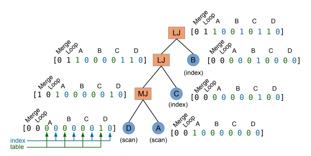
Bao, unlike Neo, encodes only the operators themselves. Otherwise, everything is the same — one-hot for the operator type (taking into account null, so that it always turns out to be a binary tree) and 2 numerical values at the end for cardinality and cost, respectively. To account for more dynamics, you can add a one-hot value for the existing cache, which, of course, will be a hint for estimating the actual execution time of the plan in real production databases.

Results

What distinguishes the article about Bao from those I have already reviewed is the volume of practical experiments on real production tasks.

1. Comparisons were made on PostgreSQL (with and without Bao), as well as on an unnamed commercial DBMS (with and without Bao).

2. IMDb, Stack, and Corp datasets were used as benchmarks — each with its own specifics for a particular case (changing the DB schema/changing the workload/changing the data).

3. And the cherry on top — real cloud servers from Google Cloud of various configurations (from 2 to 16 CPU cores + T4 GPU) were used. Both the money spent on all the used resources and the quality/speed of the model were measured.

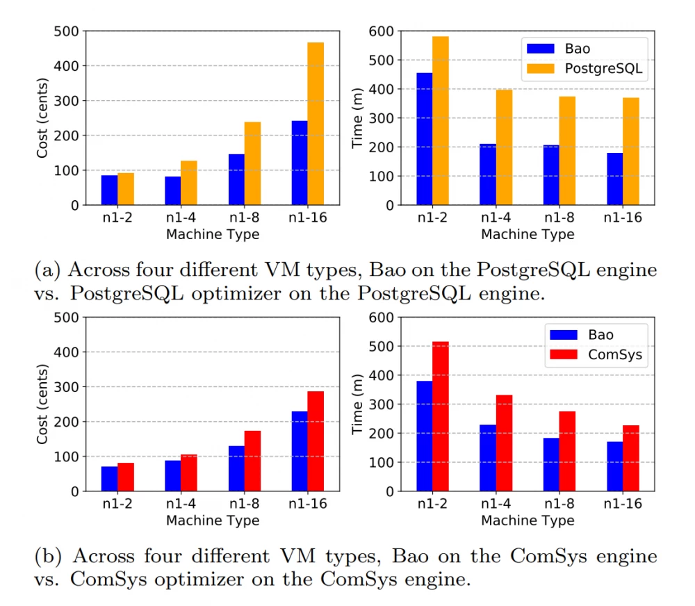
Let's look at the detailed metrics for the IMDb dataset:

The graphs on the left indicate the cost in cents depending on the server configuration and optimizer. On the right — the total runtime of each optimizer in minutes, including the time for plan formation, training, and query execution (again depending on the configuration). The overall trend is clear — Bao wins everywhere in terms of cost and speed, regardless of the cloud server configuration (2/4/8/16 cores).

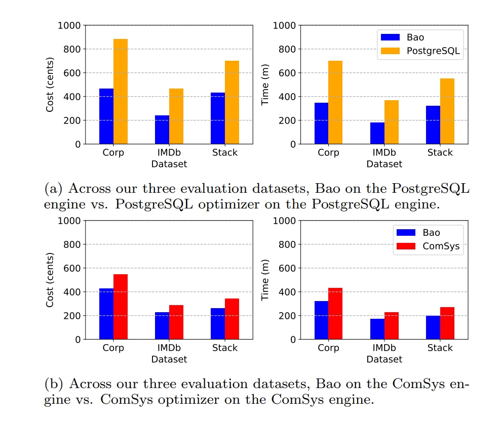
A similar picture will be observed on the other datasets (all configurations for 16 cores):

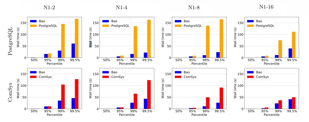
We also saw a reduction in the time spent on tail examples (in statistics, they would be called outliers):

We see that at the 99.5th percentile, the total time for query building and execution is significantly reduced.

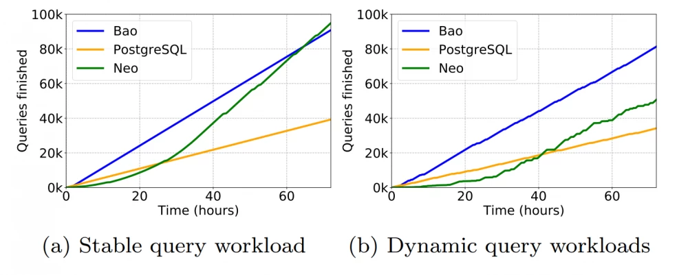
There is one final showdown with its conceptual progenitor — Neo. Let's look at the total number of requests executed when running the IMDb dataset 20 times in a row on 16 CPU cores:

On the graph on the left, the load is static, Bao immediately shows a good result, but after a while, Neo gains experience and finds more room for optimization within its E2E pipeline. However, on the right, there is already a graph for dynamic load on the same dataset. Here, Neo, firstly, takes much longer to reach the level of the standard optimizer, and secondly, does not come close to Bao's speed.

It can be said that Bao has excellently coped with the task and in every sense has brought neural network optimizers to the level of product solutions. Moreover, you can try Bao yourself using the implementation from GitHub.

Balsa

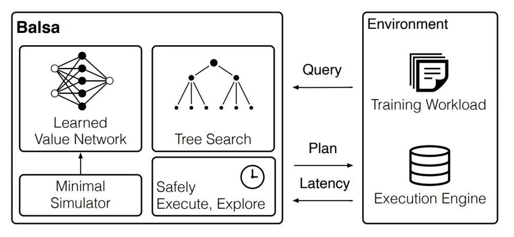
Let's leave the wonderful world of combining existing optimizers with ML models. Our next approach, Balsa, is a purely neural network optimizer. Its scheme looks as follows:

It is similar to both Neo and DQ, but nevertheless, it is fundamentally different:

The table shows that Balsa has incorporated all the most productive ideas of previous approaches but has eliminated their significant drawback - the use of expert system results. How does Balsa manage to build a plan without resorting to human developments? After all, training a policy from scratch along with executing each plan is a catastrophically slow converging process.

This is where the so-called Minimal Simulator comes into play.

Minimal Simulator

Minimal, because it uses a naive, heuristic-independent assumption for plan evaluation — the smaller the total cardinality of the plan, the better. That is, for a good plan, the value of the following cost function is minimal:

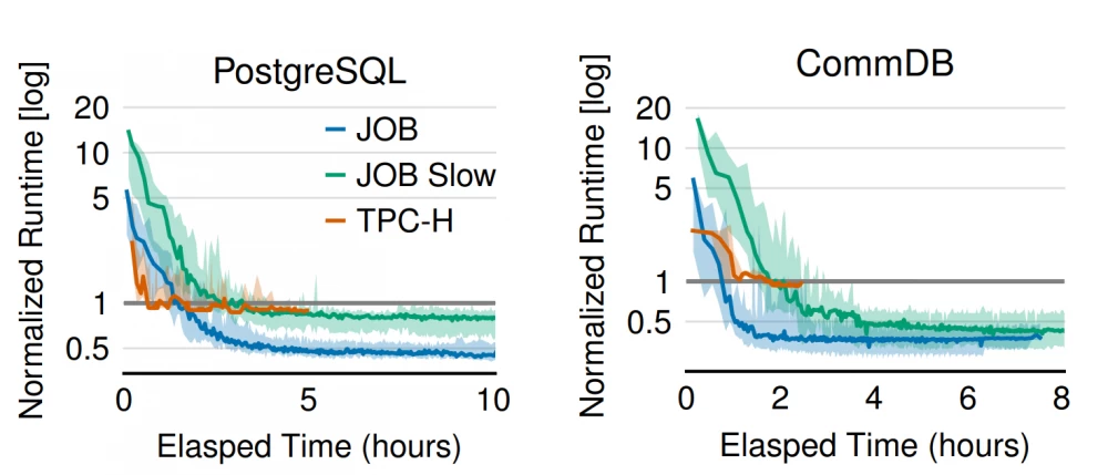
The unit in this case is the result of the standard optimizer, and the columns show the results for Balsa on train and previously unseen test, respectively. We see 3 different groups of benchmarks:

1. JOB — speed on the entire JOB benchmark

2. JOB Slow — speed on slow (edge) queries in the JOB benchmark

3. TPC-H — a benchmark for testing on artificially generated data based on uniform distribution (the scale factor parameter, responsible for the volume of generation, is 10 for the authors)

Everywhere the result on train is obviously better than on test. In any case, the network learns to generalize the found patterns and almost everywhere outperforms expert systems.

However, we remember that the convergence of RL approaches is very long, and Neo, for example, needed about a day to outperform the existing optimizer. Balsa, due to the passed simulator, does not have this problem, and it reaches a good level after 2-3 hours of work on all benchmarks:

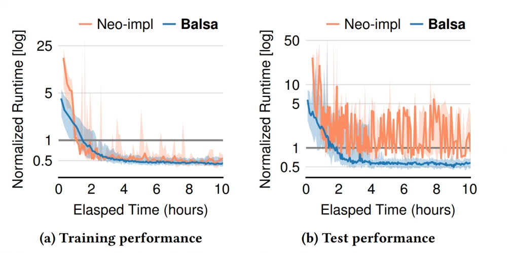
What about compared to Neo? After all, Balsa is distinguished only by the use of a simulator and the transition to an on-policy RL scheme, where the current policy is gradually retrained based on its own decisions.

A very interesting picture emerges. First, Balsa generates plans about 5 times faster in the initial iterations thanks to training on the simulator. Then on the train, they seem to be comparable, but in the test, it is clear that Balsa is much more stable and does not allow itself to build catastrophically long query execution plans, which indicates a better ability to generalize. And also, since Neo quickly accumulates an Experience dataset, on which it completely retrains the model in the process, it gradually slows down. And, for example, to run 100 iterations, Balsa took only 2.6 hours, while Neo took 25 hours! Thus, seemingly insignificant modifications significantly improve the performance of the chosen architecture.

The authors of the method did not hesitate to make a final comparison with Bao:

It is not surprising that Balsa almost always outperforms Bao, as a consequence of the greater number of degrees of freedom in RL models necessary to find the optimum. However, the natural disadvantage of Balsa in this regard remains the inability to quickly adapt to changes in the database.

AQO (Adaptive Query Optimization)

Since we are discussing production-ready solutions in the field of neural networks and machine learning in general, I cannot fail to mention a successful example of adapting and applying the classic ML algorithm K-nearest neighbors to the problem of query cardinality estimation. AQO, or adaptive query optimizer, was developed by my colleagues from Postgres Professional back in 2017, and it is still being developed within the Postgres Pro DBMS and a separate repository on GitHub.

In short, in this approach, a sample of objects is formed, the features of which are the selectivity values for each predicate of the executed SQL query (these values are taken from histograms built by postgresql). For all such objects, there are true final selectivity values collected after the execution of the corresponding queries. So we get the task of building a regression predictive model that can significantly improve the performance of the basic optimizer, taking into account the experience already lived. Different architectures were tested - both based on boosting and on neural networks, but in practice, KNN showed itself better. In general, the whole point is in the idea of representing the model itself as some unknown function, and how exactly to search for it is a matter of implementation.

There was already an article on tekkix that detailed all aspects of AQO 1.0 - for its study, I advise you to refer to it. At the moment, AQO 2.0 is relevant, which was released a year ago. It has improved performance and ease of use due to the optimization and simplification of many complex elements of the system (the corresponding changes can be seen in the presentation).

Conclusion

The bottom line is simple — ML in general and neural networks, in particular, can successfully cope with the challenges that arise in real business. Many of the approaches considered are already being developed both in open-source and in commercial DBMS, which cannot but rejoice. It remains to analyze several unique models by their nature, which make another important step in the development of neural network query optimizers — we will tell you about this in a new article.