- AI
- A
History of YOLO – the most famous computer vision architecture
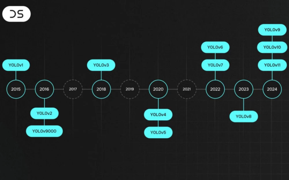
YOLO stands for You Only Look Once. It is a widely known computer vision architecture, famous for its numerous versions: the first one was released in 2016 and only solved the task of object detection in images, while the latest one – the eleventh – appeared in September this year and is already a fundamental model that can be used for classification, object tracking in videos, pose estimation tasks, etc. All of this is in real-time.
Yes, speed is exactly what set YOLO apart from other models eight years ago. Before it, there were other detection architectures in the CV world. For example, in 2015, the best was considered to be Faster R-CNN. But despite the word "faster" in its name, this model still lagged in online tests due to its cumbersome structure. Therefore, when scientists from Washington proposed YOLO, which outperformed competitors in terms of time while showing good metrics, it effectively revolutionized CV. Over the next 8 years of its existence, YOLO became a kind of transformer in the computer vision universe: it is loved and used everywhere.
This article is a full-fledged techno-history of YOLO. We will tell you what the detection task is, how the very first YOLO worked, and how it was improved in all subsequent versions.
Disclaimer: further in the text, you will sometimes encounter terms from machine learning, references to models, methods, or names. When writing, we tried to make the text understandable and interesting for both experienced readers and beginners or just interested specialists.
But if you still want to learn more about something (or someone), we recommend checking out our Data Secrets Telegram channel. We are a team of practicing ML engineers, and we have been running the channel for more than two years: every day we post analyses of ML articles and models, news, and useful materials on Data Science. So it has already turned into a kind of encyclopedia, and you will definitely be able to find something on your question :)
And now – let's go!
The detection task – how to solve it?
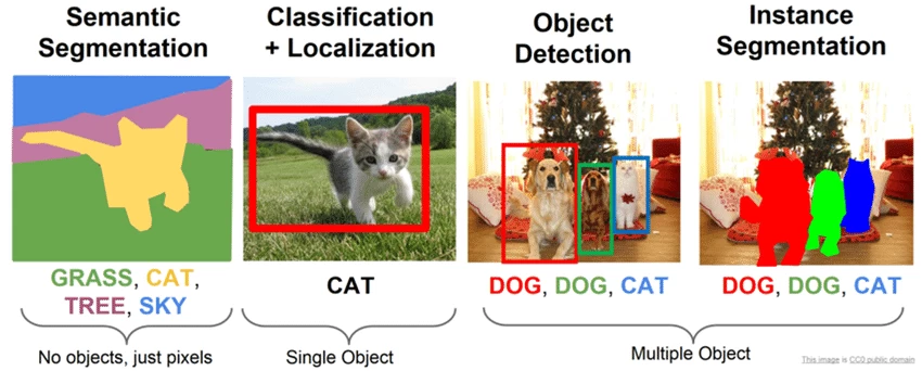
Detection is one of the subtypes of the problem of finding objects in an image. Why "subtypes"? Because although finding an object in an image seems like a clear task, if you think about it, it sounds quite vague. What does it mean to find? Just determine if there is a certain object in the photo? Find all objects in the photo? And to find – is it just to list or also to mark directly on the image? And how to mark?... It turns out that depending on the answers to these questions, the task is formally called differently:
If you need to determine the presence or absence of an object of a certain domain in the image – this is classification (classification)
If you need to perform classification, and also determine the frame that limits the location of a single object instance in the picture, – this is classification and localization (classification and localization)
If you need to determine the belonging of each pixel in the picture to a certain category – this is semantic segmentation (semantic segmentation)
If you need to perform segmentation, but at the same time differentiate only objects of a certain entity – this is instance segmentation (instance segmentation)
Detection (object detection) is traditionally called the task in which it is necessary to highlight several objects in the image by finding the coordinates of their bounding boxes and classifying these bounding boxes from a set of predefined classes. At the same time, unlike the task of classification with localization, the number of objects in the image is not known in advance.
Frames in which objects need to be enclosed are called bounding boxes or simply b-boxes. B-boxes traditionally have a rectangular shape and are positioned so that the sides of the rectangle are parallel to the image frames. It is also intuitively clear that the frame should be "minimal", that is, capture the object completely while having the minimum area. How we define the b-box depends on our architecture, but usually one of two options is chosen: center coordinates (x0, y0) + width (l) and height (h), or the coordinates of the top left pixel (x1, y1) + the coordinates of the bottom right (x2, y2).
Note that in the detection task, the model must be able to solve two problems at once: finding the optimal b-boxes and classification. The most naive approach that comes to mind is to iterate over all possible b-boxes and run each of them through a convolution-based classifier. But it is well known that almost any exhaustive search is an impossibly long and inefficient process. Therefore, in real architectures, it is slightly tweaked. For example, there is a group of methods called two-stage, which at the first step select only some b-boxes, with a high probability of containing an object, and at the second step, such selected frames are fed to the classifier. These methods include R-CNN and its descendants Fast R-CNN and Faster R-CNN.
YOLO, on the other hand, became the first representative of another group of methods - single-stage algorithms, in which a separate model for region selection is not used at all. Instead, YOLO is a single network that immediately predicts the coordinates of a certain number of b-boxes along with their characteristics, such as class probability.
YOLOv1
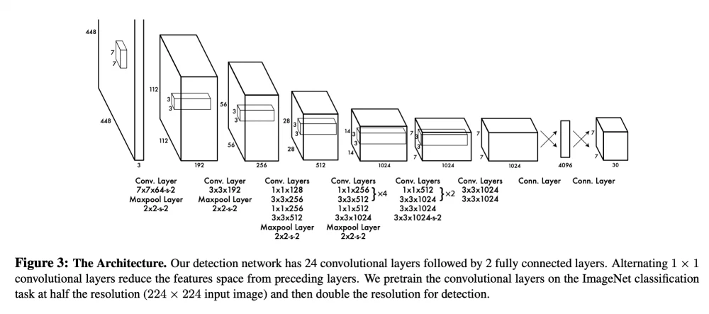
So, the following architecture is at the core of YOLOv1:
This is a slightly modified GoogLeNet: in the original CNN there are 22 convolutional layers, but the creators of YOLO added two more + fully connected layers at the end. The input to this network is an image of 448x448 (yes, if you submit an image of a different size, it will simply be cropped and/or sent to the resize function), which was previously divided into equal square cells of size 64x64 in such a way that it turns out to be a 7x7 grid (no, 7x7 is not a magic constant, you can use a different cell size, but how it will affect the network has not been particularly studied). We need the cells so that all operations further take place at the "cellular" level. This is the main innovation of YOLO: its creators were able to formulate and solve the detection problem as a regression problem.
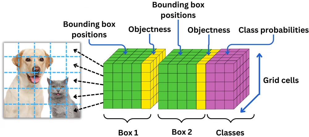
If you look at the last layer of the diagram, you will notice that the output tensor of the network has a size of 7x7x30. That is, for each of the 7x7 cells of our image, the model predicts a vector of 30 numbers. Inside this vector lies the description of the b-boxes and class labels. More precisely, the first 10 values are responsible for the coordinates of the two candidate b-boxes: center coordinates + width + height + confidence score, that is, the model's confidence that the center of the object is inside the b-box. The remaining 20 values of the vector are responsible for the class labels, that is, the probability estimate that an object of a certain class is present in the cell. Why 20? Because that was the number of classes in the original dataset.
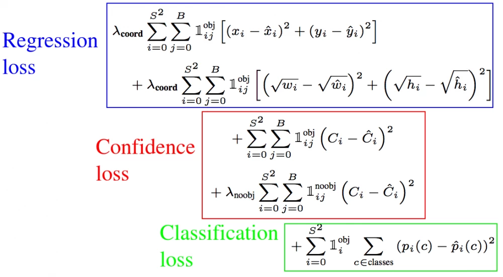
That's all for the architecture. Now let's see how it is trained. It should be mentioned that before training the model completely, the researchers first fine-tuned the last 4 layers on image size 448x448 (unlike the first 20 classification layers trained on 224x224 ImageNet). But let's get back to the main YOLO loss. It is a complex combination of classical classification and detection losses and looks quite intimidating:
Let's break it down into parts. The first part, marked as regression loss, is quite simple. It is the error in predicting the coordinates of the center (x,y), height (h), and width (w) of the bounding boxes. The index i stands for objects, and the index j stands for boxes. The bold beautiful unit here is an indicator function that allows considering only the cells that contain objects and only the contribution of the considered bounding box j (if it is the same object i, but a different box, the expression will be zeroed out to avoid counting the same error twice). As for the roots applied to the height and width of the bounding boxes, this is simply a scaling measure necessary to penalize small bounding boxes more for not matching the actual markup.
The last part – classification loss – is also clear. This is a classic quadratic loss, where we calculate errors on those very twenty class labels. At the same time, the indicator function here again ensures that only those cells that actually contain an object are taken into account. We also consider cells without objects further, but for the loss, it is important to maintain balance, and since most cells will not contain objects at all, cells containing anything need to be given more weight.
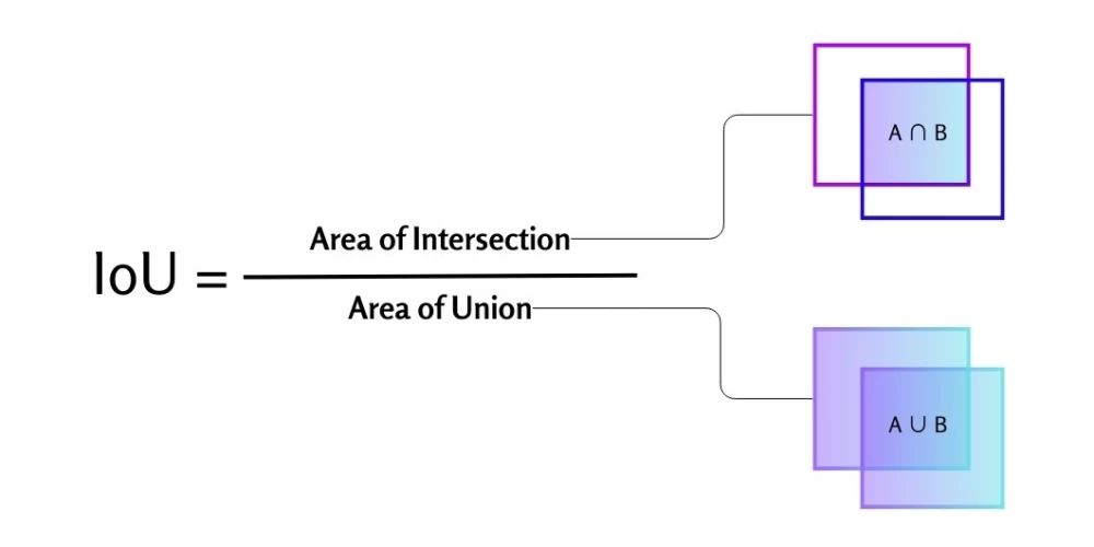
Finally, Confidence loss. This is the part of the loss function that is responsible for the model's "confidence" estimates that the center of the object is inside the bounding box (they are marked in yellow in the previous diagram). At the same time, this is not just a probability. This is the predicted value of the IoU function, that is, Intersection over Union. This is one of the defining metrics of computer vision, and it is easiest to understand it by simply looking at the picture:
In terms of bounding boxes, IoU is the overlap between the predicted frame and the true rectangle from the train. It turns out that if the model predicts a high IoU, it "believes" that the overlap will be large, and, in other words, is more confident in the existence of a certain bounding box. Conversely, if it predicts a low IoU, it is confident that there is no object in the cell at all. That is why this part of the loss also takes into account cells that do not contain objects (a beautiful unit with the index noobj): we teach the model to give fewer false positives on them. We weigh such cells using the constant λ_noobj, which is usually about 10 times smaller than λ_coord.
Thus, our loss function "teaches the model" to correctly position the bounding boxes in space and estimate their size, correctly classify the found objects, and also simply accurately determine the fact of the presence of an object in the cell and thereby not overfit.
So, we also figured out the train. The non-obvious part remains: inference. Suppose we trained the model, and it gives us some tensor as output. How to assemble the final answer from it, which should contain filtered bounding boxes with class labels?
First, you need to link class labels to specific b-boxes. After all, in each output vector, we have two boxes, and the probability for each class is only one. To link them, you need to take the confidence score of each b-box and multiply it by each class probability. This way, we will branch out our classification labels and end up with 7 * 7 * 2 = 98 rectangles, each of which has class labels, center coordinates, width, height, and IoU aka confidence score.
Now we need to decide which of the b-boxes we will keep and which we will delete. To do this, we will simply delete all boxes for which IoU < 0.5 (that is, those that the model is more likely to think do not contain an object).
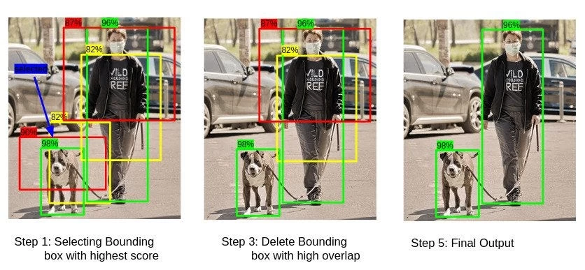
But that's not all. After all, an object may not fit entirely into just one of the cells we defined at the very beginning. Then two, or even three b-boxes from different cells may actually be a single b-box for the same object. This is where the Non-maximum Suppression algorithm comes to the rescue. It is quite simple and elegant. First, we take the list of b-boxes that remain after step 2 and sort it in descending order of IoU, so that the b-boxes that the model thinks contain the centers of objects are at the top. Then we will sequentially take the most "probable" candidates and find all the b-boxes that intersect with them so much that the IoU of this intersection is greater than a certain threshold. All such b-boxes will be deleted and crossed out from the original list, and so on until the list is empty and we have a set of final filtered b-boxes.
That's all. This is how the first version of YOLO worked.
The model, of course, turned out to be amazing and caused a sensation in 2016. But it must be said that at first, it did not win the audience's sympathy. Although the model was very fast and worked in real-time, it had problems with metrics (63.4% on PASCAL versus 73.2% for Faster R-CNN), and it did poorly with overlapping objects. However, researchers later fixed this. Let's see how.
YOLOv2
The authors of the article about YOLO quickly realized the shortcomings of their model and released the next version – YOLOv2, as well as a small extension – YOLO9000, just a few months later. The model not only advanced in metrics but also became even faster than the previous version and learned to recognize 450 times (!) more classes – hence the 9000 in the name.
But let's go step by step again. First, the architecture.
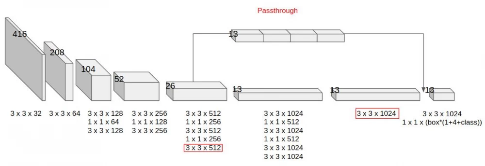
Fully connected detection layers were removed from it at the end. Convolutions took their place. In addition, dropout was removed from the architecture. Instead, batch normalization was added, which at that time proved to be a good tool for improving the convergence and training speed of the model.
The basic architecture itself was also changed from GoogLeNet to Darknet-19. This network consists of fewer layers: 19 convolutional layers versus 22 in GoogLeNet. Due to this substitution, the model did not sag on real-time tasks.
If in the previous version the first 20 classification layers were retrained on 224x224 images from ImageNet, then the second version was trained on higher quality images: 448x448.
At the same time, during the training of the entire architecture, the resolution of the input image was reduced to 416x416. This was done for a reason. The fact is that in this case the image can be divided into an odd number of cells: then in the middle of the image, where the probability of an object appearing is highest, there will be one cell, not four.
The number of cells has also been increased. If in YOLO1 we mentally cut the image into a 7x7 grid, now it was a 13x13 grid. Technically, this was implemented by removing one pooling layer, resulting in an output tensor size of 13x13x125.
Why 125? Because in YOLO2 we predict class labels not for all cell boxes at once: now each b-box has its own vector of such probabilities. Moreover, now there are more b-boxes per cell: previously there were two, and now the number has increased to five. A total of 5 b-boxes, for each the coordinates of the center, width, height, IoU and 20 class labels: a total of 125.
Skip connection layers have appeared, which prevent the model from overfitting and make it more stable. The idea here is that the data is duplicated, and the first part of it passes through certain layers of the network, and the second part kind of skips them. At the same time, this "lazy" part, in order to maintain the output dimension, is simply divided in certain proportions and added to its twin, which has passed through a certain number of convolutions.
The listed is far from the end. In YOLO 2, the very idea of the approach to object detection has changed. Instead of traditional bounding boxes, the researchers drew from Faster R-CNN the idea of predicting anchor boxes (or anchors). Recall that Faster R-CNN is a two-stage method, and before the input data is fed into the classifier, the network already has a bunch of candidates for the final bounding boxes. Therefore, Faster R-CNN, unlike YOLOv1, does not have to predict coordinates from scratch: it only predicts the shifts needed to move the original boxes. This task is much simpler and more reliable in terms of accuracy, so it was decided to add candidates (priors anchors) in YOLOv2, which we will then learn to move.
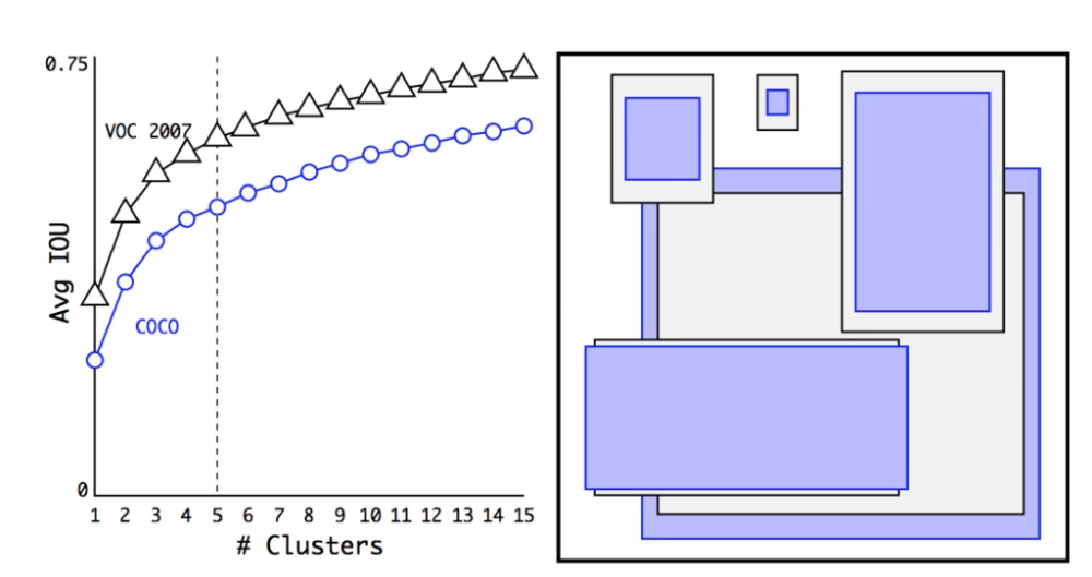
The researchers chose the shape and number of initial anchors in a very interesting way. To do this, they turned to the labeled COCO and VOC datasets and, roughly speaking, compiled statistics on them. In each of the datasets, all existing bounding boxes were clustered using the K-means algorithm (only instead of Euclidean distance, IoU was used as a measure of proximity), and calculated after how many clusters the accuracy reaches a plateau. It turned out that after K = 5, mAP is already 61%, and then it grows not very much. Then, in each of the five resulting clusters, the average bounding box was taken, and so those 5 anchors were obtained, for which we will make predictions in each of the 13x13 cells of the image.
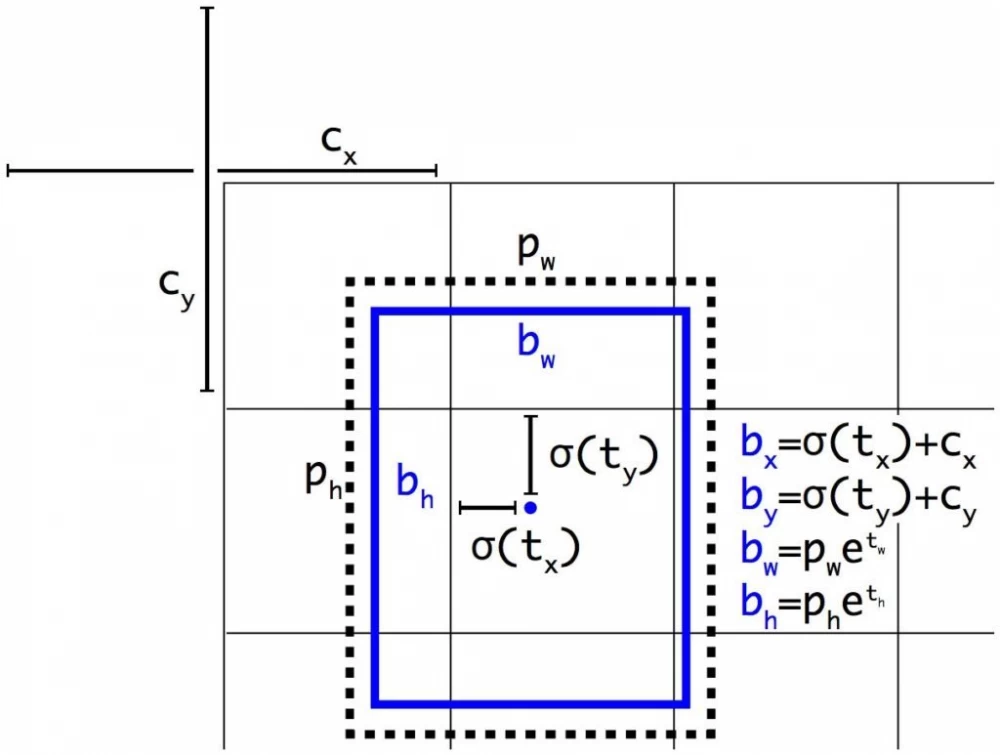
So, are the vectors that are output for each cell now interpreted differently? Yes. As we mentioned earlier, the size of the output tensor in YOLOv2 is 13x13x125: 5 anchors, for each 20 class labels, confidence score, and four more features. Previously, these four features were the coordinates of the center, width, and height of the bounding box. Now it is a set of numbers t_x, t_y, t_w, t_h, which are responsible for shifting the anchor left/right, up/down, changing the width and height, respectively. The final coordinates of the bounding box are calculated according to the following logic (here c_x,c_y are the coordinates of the top left corner of the cell, p_w, p_h are the original height and width values of the anchor):
Sigmoid and exponential functions are used here to stabilize training, so that the network's predictions are immediately calculated only relative to a specific cell, rather than the entire image.
There were no changes in training as such. Still the same loss, still calculating IoU, and applying Non-maximum Suppression at the end.
What about YOLO9000? Wasn't it supposed to have 9000 classes, not 20? That's right, these 9000 classes are actually the 9000 best classes from ImageNet, combined with classes from COCO. However, to combine these two datasets, researchers had to work hard: the fact is that ImageNet has more classes and they are more specific. For example, if ImageNet had classes like "doll", "teddy bear", "ball", in COCO it was all just called "toy". To get around the problem, a whole tree structure of classes was created. During the test, we follow from the top to the root, and it is at the root that we calculate the metrics, avoiding class exclusion and related network collapses. At the same time, in this version, the number of anchors per cell was reduced to three, so that the size of the output tensor was not too large.
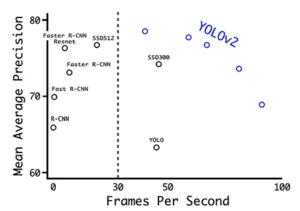
What is the result? As a result, YOLOv2 is already becoming SOTA on PASCAL VOC and COCO. The network outperforms all competitors in metrics and speed, can work on various image sizes and in real time. At 67 FPS YOLOv2 gives mAP 76.8, and at 40 FPS – 78.6 mAP, which is much better than Faster R-CNN and SSD.
In general, faster-higher-stronger. But the researchers did not stop there. Two years later, they released the third version of the model.
YOLOv3
YOLOv3 is the latest version of the model, on which its creator Joseph Redmon worked, and the last paper on YOLO, in which he is listed as a co-author. Subsequently, he left the project because he suffered from the widespread use of his model in the defense sector. There were no loud changes in YOLOv3, it is rather a refinement of YOLOv2 and error correction.
Firstly, in YOLOv3 the authors became bolder and instead of Darknet-19 they use Darknet-53 – a much deeper network (53 convolutional layers). More layers – longer work, so the speed of the model has slightly decreased. But it was possible to achieve a very significant increase in metrics.
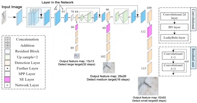
Secondly, YOLOv3 now outputs not one large tensor, but a total of three.
The image clearly shows that the architecture structure is somewhat pyramidal (by the way, in the article the authors refer to Feature Pyramid Networks). The first feature map we get has the usual large size of 13x13 (high level features). The next one is smaller – 26x26 (middle level features). The last one is very small – 52x52 (low level features). The meaning of this division is that the smaller our grid, the smaller objects the model can find. For larger objects, it is easier to use a large division. And if we have both, the network can work at different levels and catch objects of large, small, and medium sizes well.
There were also some small changes to the loss function. The Confidence score became the objectness score. There are no conceptual changes here – it is still the degree of confidence of the model that there is a b-box in the cell. But there is a nuance: it is no longer quite IoU, rather IoU with normalization. The objectness score, unlike the Confidence score, must be equal to one for the b-box in which the model is most confident (that is, for the box with the maximum intersection with the true frame among all predicted b-boxes). And the parameter was not just renamed, now it is reflected differently in the network loss. The updated loss function looks like this:
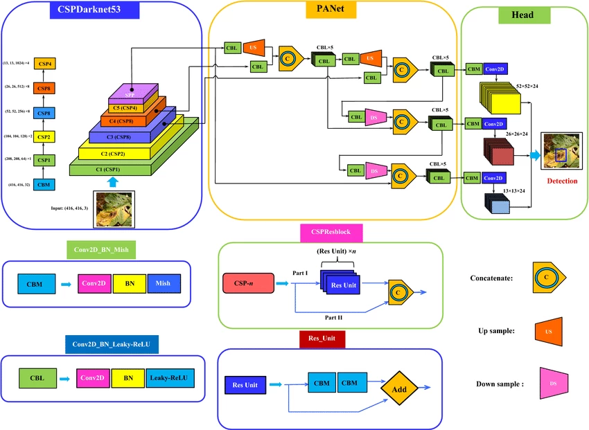
The approach to building the pyramidal structure of the network has changed. The authors noticed that although the method with three feature maps improved the model's performance on small objects, the quality on large objects, on the contrary, decreased because the largest output of the model does not go deep enough into the network and learns somewhat superficially. To solve this problem, the authors added additional "enrichment" layers to the model (in the diagram below, this is the PANet area). Also, pay attention to the lilac layer in the blue area, which is called SPP. This is also a new element of the network – Spatial Pyramid Pooling. In fact, this is again an analogue of skip connection: several pooling layers are applied to the original image in a heap so that a little more information about the original context remains in the features at the output of Darknet.
The method for calculating the final coordinates of b-boxes is taken from YOLOv3, with the exception of a small change. The change consists in adding a normalization constant. The fact is that it turns out that the formulas for calculating the coordinates and sides from version 3 go a little "crazy" if the center of the object is close to the edge of the cell. When normalization is added, the problem is leveled.
Finally, the post-processing algorithm, which has not changed since the first version, has undergone changes. Instead of Non-maximum Suppression, Distance-IoU Non Maximum Suppression was now used, which, as you can guess, differs from the classic NMS by using the Distance-IoU metric instead of the usual IoU. Distance-IoU, in addition to directly overlapping the frames, also takes into account the distance between their centers.
We have listed 5 main changes that were added to YOLO4. In addition, the researchers experimented with many other tricks and added small useful features to the model, such as a scheduler and Cross mini-Batch normalization, selected the best hyperparameters of the model, and even tried to integrate the attention mechanism into individual layers of the network.
Thanks to the work done by the authors, YOLO has become 20% better than its previous versions and has again broken into SOTA, while maintaining speed.
YOLOv5
YOLOv5 is a Cinderella or Ugly Duckling story in the computer vision universe.
It appeared extremely soon after YOLOv4. Only a month has passed! "Isn't this too fabulous a pace to be true?" you may ask. Yes, it is. Until now, each new model was truly new and brought many fresh ideas, changes in architectures and approaches to detection. However, YOLOv5 seemed to the YOLOv4 community to be just rewritten in PyTorch. Even a scientific article did not come out with the implementation of the model. Yes, it should be mentioned that none of the authors of the previous models were involved in the creation of YOLOv5 - the new version was released at that time by a not very well-known company Ultralytics. The company promised to release an article within a few months, but... 4 years have passed, and there is still no article.
This is not all. The reputation of the model was also quite tarnished by the fact that in the originally published metrics, which were released by another company, Roboflow, there were errors. Incorrect measurements of model speeds were made, and, as a result, the metrics and graphs did not reflect the real picture. Many researchers and engineers were so upset with the version that they even said it was not worthy of the title YOLOv5.
And, by the way, for some time Ultralytics did indeed plan to change the name, but... it was somehow forgotten. The company managed to get away with it, and although they did not release the article, they made at that time one of the most modern platforms for fine-tuning and working with YOLOv5 in general. And they also promised that they would work on improvements. And they did not deceive: for two years they diligently worked on the model and the ecosystem, even released an application.
Yes, during this time, the researchers at Ultralytics have done a really great job: they updated some blocks of the model (in particular, they added more C3 blocks, replaced SPP with SPPF), changed the activation, added successful weighting of different feature maps to the loss, came up with many new augmentations and engineering tricks to improve performance. All this helped to increase mAP by as much as 6%, and in combination with the MLOps environment, which Ultralytics also constantly updated and maintained, YOLOv5 became a real favorite! Many still use this version, and the company still constantly updates it.
YOLOv6... or v7?
Actually, it would be fair to first talk about YOLOv7. It unexpectedly came out two months earlier than the sixth version (in July 2022). Why? Simply because different laboratories were involved in the development, which, apparently, could not agree on the timing and names...
Here it is necessary to make a small lyrical digression and say that in two years, in addition to improvements to YOLOv5, different groups of scientists managed to do a lot for this architecture: YOLOX, YOLOR, three versions of PP-YOLO, and many other small variations of the model were released. Apparently, after the story with the fifth version, everyone was afraid to call the model v6 :)
And, by the way, the sixth version did not become as popular as the fifth. Here are the changes proposed by Chinese researchers:
In YOLO 5, a trend was set for publishing models of different sizes, but they only differed in the number of parameters. In YOLOv6, it was proposed to slightly change the basic backbone for models of different volumes. For small models, RepBlock was used, and for larger models, CSPStackRep was used.
The loss was also updated again in the model: now it did not take anchors into account, because the model was made without anchors at all. This idea was borrowed from YOLOX and is called Anchor-Free Decoupled Head. We returned to the approach from the first version: predicting the coordinates of the center of the rectangle and the lengths of its sides. And the problems that were associated with it were solved using the idea from the fourth YOLO - adding normalization relative to the cell.
Scientists also proposed using Efficient Decoupled Head and many tricks to speed up the model. What did not appear there: Task Alignment Learning, distillation, quantization, and reparameterization.
YOLOv6, by the way, just like YOLOv5, is still constantly being updated and used, but mainly only in China. An interesting fact: this year its creators have already released the sixth version of the sixth version.
And in the seventh version of YOLO, although it came out earlier, the updates were somewhat more interesting. Alexey Bochkovsky (the one who created the fourth version) and the creator of the YOLOR version took part in its creation. As you can see, the team turned out to be strong. What did they propose?
Firstly, extended layer aggregation. This is rather an engineering trick that allows the network to learn and work faster. But it also affects the quality of training, because the aggregation layers kind of "shorten" the gradient path through the network during the backpropagation process, and scaling occurs faster due to this.
Secondly, new scaling and reparameterization techniques. The scaling idea is similar to what Chinese colleagues proposed, only here the block parameters change depending on the size of the model not randomly, but taking into account the depth of the network, the width, and the resolution of the incoming images.
Thirdly, a new Coarse-to-Fine head in addition to the three existing ones. This head is designed to control overfitting by directly influencing the loss, unlike the other heads that go through some aggregation blocks.
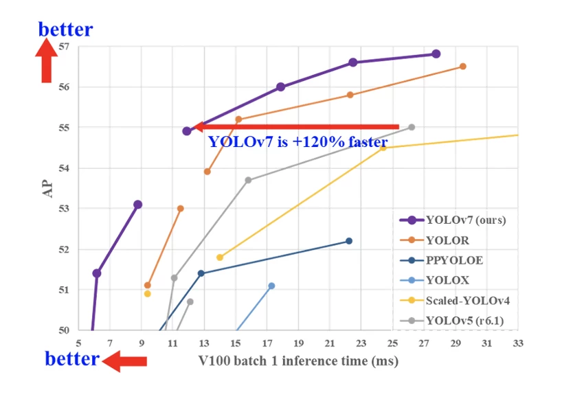
As a result, the sixth version still lagged behind the seventh, which became the new SOTA in terms of speed and quality of detectors at the time of release.
YOLOv8 – the most widely used model in the lineup
In early 2023, Ultralytics returned to the scene, but this time not with another version of YOLOv5, but with the new YOLOv8. But before talking about the model, let's talk about what made the eighth model so popular. It's not the architecture, not the fantastic metrics, and not even the lightning-fast inference. It's a completely new repository built as a unified platform for training detection, segmentation, and classification models. The company released five models, each of which can work with all the listed tasks. Among them were the small and nimble YOLOv8 Nano and the large and most accurate YOLOv8 Extra Large (YOLOv8x). All models support many export formats and can work on both CPU and GPU. And YOLOv8 also has the most convenient API, which is compatible with both the command line and Python.
There were few changes in the model itself: a new Backbone network, loss function, and Anchor-Free head. To enable the model to perform different types of tasks, it was trained in several stages on different datasets. The detection checkpoints were trained based on COCO detection with a resolution of 640. The segmentation checkpoints were trained on COCO segmentation datasets with the same resolution. And for classification, the dataset has not changed since the first version, it remains ImageNet. By the way, in the eighth version, the classification layers are again trained at a size of 224.
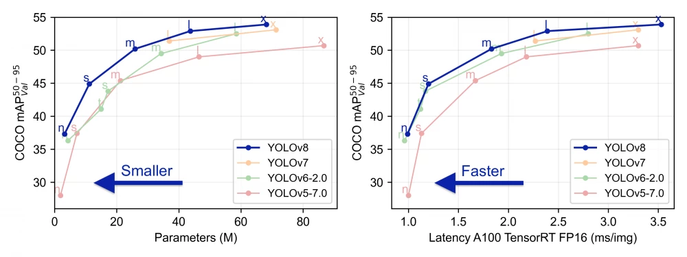
And of course, there are SOTA metrics. Look at how much better the new version performs compared to the previous ones:
Subsequent versions
All subsequent versions: YOLOv9, YOLOv10, and YOLOv11 were also released by Ultralytics, which now has an unofficial "monopoly" on this architecture. The latest version was released very recently: in October of this year. However, now the YOLO update has become more of an engineering task rather than a research one. Time after time, developers optimize inference, reduce the number of model parameters, work on model compatibility with new hardware, and improve the API.
The metrics have also been gradually improving all this time, but rather due to minor fixes rather than key changes in the architecture. For example, in YOLOv9, researchers refined the idea of layer aggregation and introduced the use of GELAN – a general aggregation network, as well as added smart gradient checkpointing – PGI.
Today, YOLO is the most accurate and efficient model, widely used for a wide range of computer vision tasks. It is one of the few deep learning architectures that remains beloved and applicable many years after its discovery.





Write comment