Autoencoders in simple terms

Autoencoders are called autoencoders because they automatically learn to encode data into a more compact or low-dimensional representation and then decode it back into its original form. This term can be broken down as follows:

• Auto: means that the process is automatic. The model learns by itself, without the need for explicit labels or human intervention to extract features. During training, it automatically finds the best way to represent the data in a low-dimensional form.

• Encoder: the first part of the model, the encoder, compresses or encodes the input data into a smaller, compressed form. This stage involves reducing the dimensionality of the input data, effectively learning a more compact version of the data.

• Decoder: the second part of the model, the decoder, attempts to restore the original input data from the encoded representation. The goal is to ensure that the output data is as similar as possible to the original input, showing that the encoding preserves the main features.

So, first of all, an autoencoder is a type of neural network used for unsupervised learning. But not just any kind, one that can encode and decode data, similar to a ZIP archiver that can compress and decompress data. In machine learning, it is used for dimensionality reduction or data compression, as well as for removing noise from images (we will talk about this later).

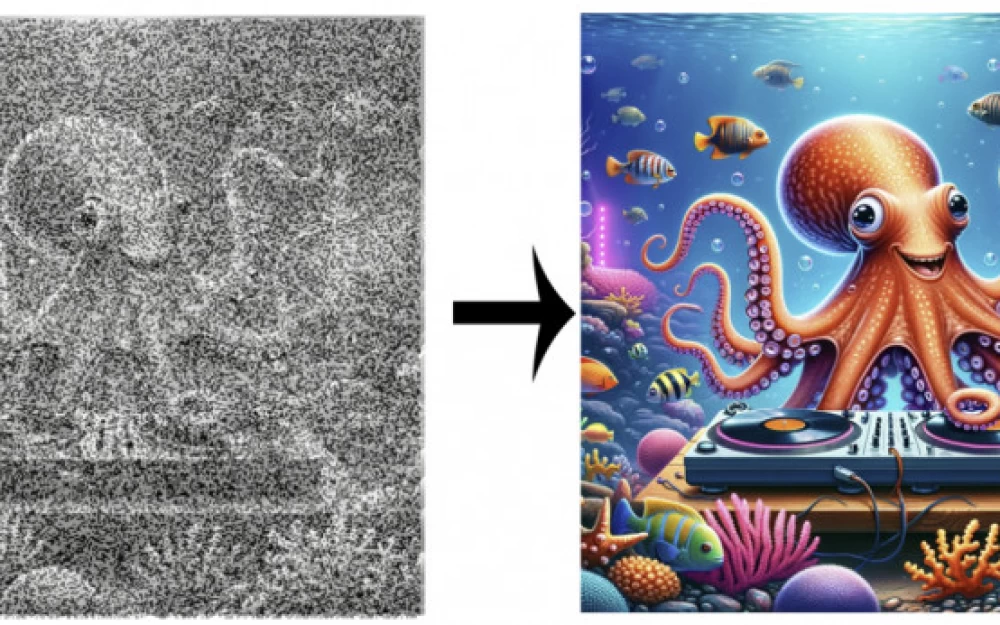
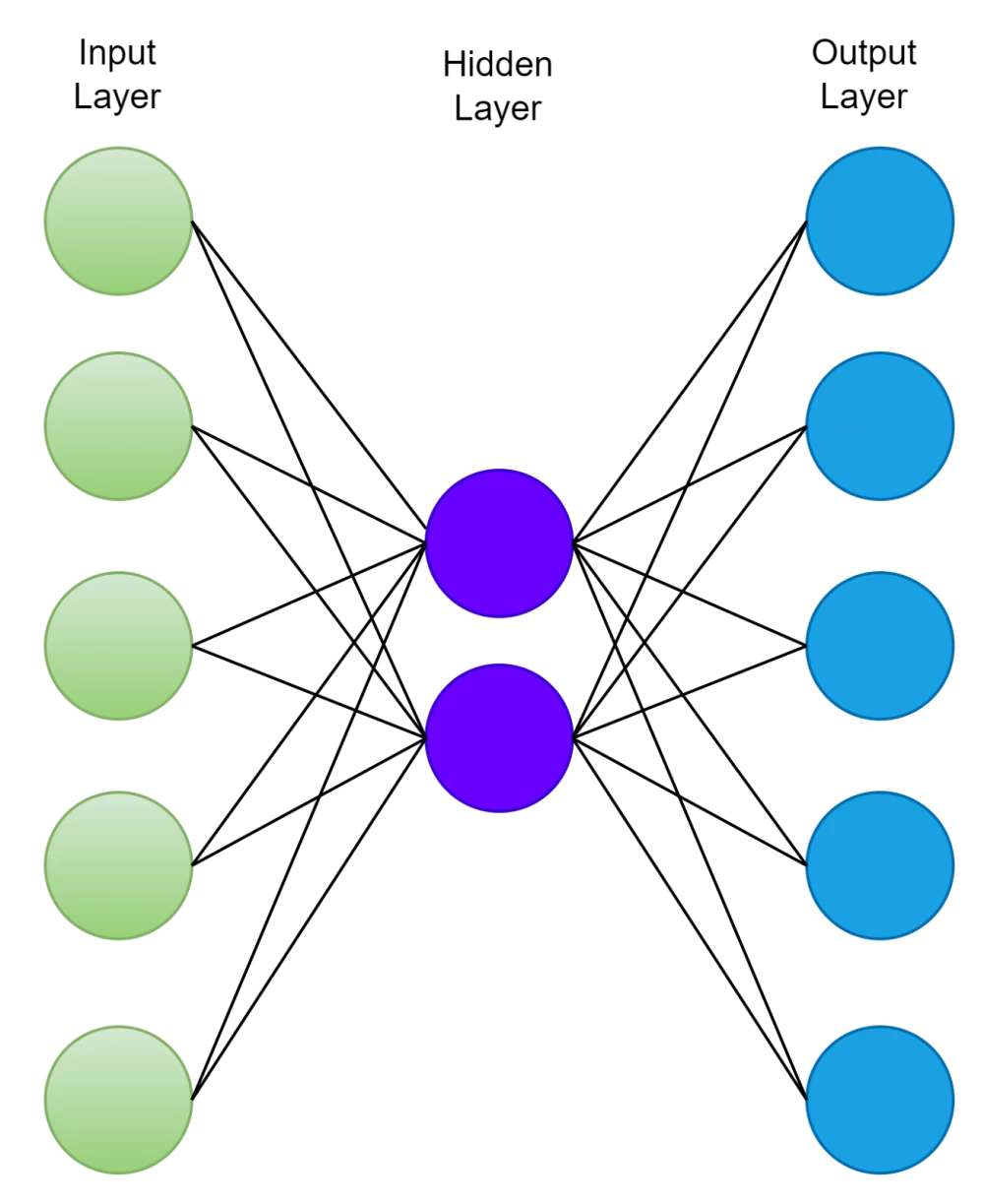
However, it does this more intelligently than a ZIP archiver. It is able to understand the most important features of the data (so-called latent, or hidden features) and remembers them instead of all the data, in order to then reconstruct something close to the original from an approximate description. In images, for example, it can remember the outlines of objects or the relative position of objects to each other. This allows for interesting lossy compression. It works roughly as follows:

Only in latent features the values are actually discrete, so the process is closer to the following:

This approach is important for diffusion models because it allows them to work in a lower-dimensional space (the so-called latent space), which is much faster than working directly with high-resolution images. That is, instead of performing the denoising process directly on the pixels, the image is first compressed into the latent space using an autoencoder, and the diffusion process takes place in this lower-dimensional space. After diffusion, the decoder restores the high-resolution image from the latent representation. If you think about it, this makes perfect sense. For the diffusion model to work, it only needs to know the main features of the original image, not all the fine details, so why waste time and computational resources on them?

The idea behind the autoencoder is a very simple trick. If we artificially limit the number of nodes in the autoencoder network and train it to restore data from the original, this will force the network to learn a compressed representation of the original data simply because it will not have enough nodes to remember all the features of the data. It will have to discard most of the insignificant features. This is, of course, only possible if there is some structure in the data (for example, correlations between input features), because then this structure can be learned and used when the data passes through the bottleneck of the network.

This network can be trained by minimizing the reconstruction error, which measures the differences between our original data and the reconstructed image after decompression.

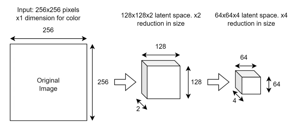
Here is an example of how the compression stage works:

At each compression stage, we halve the image dimensions but double the number of channels the network can use to store latent features.

Decoding works in reverse:

Note that in the end, we get a reconstructed image, not the original. They will be similar but not identical! Yes, the goal of the training process is to make them as similar as possible (i.e., minimize the reconstruction error), but some details will be lost.

The ideal autoencoder model finds a balance between:

1. Sufficient sensitivity to the input data for accurate reconstruction.

2. Sufficient insensitivity to avoid simply memorizing or overfitting the training data.

In most cases, this is achieved by setting a loss function with two components: one term that encourages the model to be sensitive to the input data (e.g., reconstruction error), and another term that prevents memorization or overfitting (e.g., regularization term). This is a very important observation — it is important to ensure that the autoencoder does not simply learn an efficient way to memorize the training data. We want it to find latent features to be useful for data different from the training set.

There are other ways to create a bottleneck in the network besides limiting the number of nodes.

Sparse autoencoders

We can constrain the network by limiting the number of neurons that can activate simultaneously. This will essentially force the network to use separate hidden layer nodes for specific features of the input data (an idea somewhat similar to how different areas of the brain process different types of information).

Sparse autoencoders apply regularization methods that encourage hidden units (neurons) in the network to maintain a certain level of sparsity, meaning only a small portion of them should be active (i.e., have a non-zero output) at any given time. Here are the main types of regularization used in sparse autoencoders:

Regularization using KL divergence:

The most common method of regularizing sparse autoencoders is to impose a sparsity constraint on the activations of the hidden units using Kullback-Leibler (KL) divergence.

The idea is to compare the average activation of a hidden unit with the desired level of sparsity, usually denoted by a small value (e.g., 0.05). KL-divergence penalizes deviations from this desired level of sparsity.

This is achieved by adding a sparsity penalty term to the overall cost function. The cost function becomes a combination of reconstruction error and sparsity penalty.

The desired sparsity is often denoted as p (a small value, e.g., 0.05). The average activation of hidden unit j over the training examples is denoted as pj.

The overall cost function J with regularization through KL-divergence looks like this:

Where:

• J_reconstruction — reconstruction error (e.g., mean squared error).

• β — weight to control the strength of the sparsity penalty.

• n_h — number of hidden units.

L1-regularization:

L1-regularization encourages sparsity by penalizing the absolute value of the weights, which leads to many weights being shifted to zero.

By adding the sum of the absolute values of the weights to the cost function, this form of regularization effectively encourages the model to use fewer connections, leading to sparse activations in the hidden layer.

L2-regularization:

L2-regularization, also known as weight decay, discourages large weights by penalizing the sum of the squares of the weights.

Although L2 regularization does not directly ensure sparsity, it helps prevent overfitting and can complement other methods that promote sparsity, such as KL divergence or L1 regularization.

Activity Regularization:

This method directly penalizes neuron activations. A term is added to the loss function that penalizes non-zero activations, often computed as the L1 norm of the activations.

By minimizing the sum of activations, such regularization encourages most neurons to remain inactive.

Denoising Autoencoders

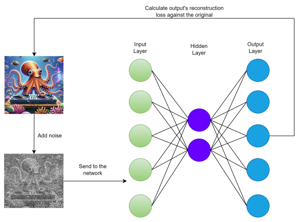
Another idea is to add noise to the original image and use it as input, but for error calculation, compare it with the cleaned original. Thus, the model learns to remove noise from the image, but as a side effect, it can no longer simply memorize the input data because the input and output do not match. Here is what the training process looks like:

This, as mentioned above, forces the model to memorize only important features and ignore noise (and other insignificant details).

Variational Autoencoders (VAE)

They are used in diffusion models. The main idea is that in regular autoencoders, features are stored as discrete values in feature layers. In variational autoencoders (VAE), a probabilistic distribution is used for each latent feature. This allows the network to implement some interesting functions that I will describe in a separate article.

Limitations
Since autoencoders learn to compress data by identifying patterns and relationships (i.e., correlations between input features) that emerge during training, they tend to effectively reconstruct data similar to those used in the training process.

Also, the ability of autoencoders to compress data is rarely used by itself, as they usually are less efficient compared to manually created algorithms designed for specific types of data, such as sound or images.

Although autoencoders can be used for text encoding, they are less frequently applied compared to more modern architectures such as transformers (BERT, GPT, etc.), because autoencoders may struggle with processing complex language structures or long sequences, especially without mechanisms like attention that help capture long-range dependencies.

Conclusion
Autoencoders are fundamental building blocks in the field of machine learning and AI, offering a versatile approach to tasks such as data compression, dimensionality reduction, and noise removal. By learning to encode data into compact, low-dimensional representations and then decode them back, autoencoders can effectively capture important features of the input data while discarding less significant details. This capability makes them valuable in applications ranging from image processing to data preprocessing, as well as components of more complex architectures such as latent diffusion models.