Traffic Under the Microscope: ML Model in Search of New Network "Fingerprints" of Malware

But the machine learning team did not stop there. Together, we conducted a series of new experiments, expanded the input feature set, and tested the model on more complex scenarios, leading to an update of the model and an even higher detection rate.

In this article, we will detail the updated features of our model, their technical implementation, and how they are integrated into the developed ML model. You will learn about the challenges we had to solve, the mistakes we had to correct, how and why we changed the feature set, and what new threats we were able to catch as a result.

Happy reading!

Brief Introduction: Key Changes in the ML Model

Regarding the approach described in our previous article, we have revised the formation of the model's feature set. The initial solution was based on expert knowledge about the behavior of the target variable, which made the feature set more point-specific. That is, one-hot features were constructed for specific values of interest to us. This allowed us to maintain high interpretability of the model's verdicts and to control its behavior more finely on individual samples. However, over time, we have managed to accumulate enough data from various sources to be able to fully rely on our sample, trusting the representativeness of the distributions. As a result, we were able to restructure our feature set from a point-based expert nature to a statistical one based on data.

Analysis of Updated Features with Examples

For clarity on the changes and the influence of features on the model, we will look at SHAP values. As an example, we will look at two features — one relates to the Content-Type header in the HTTP Response, and the other relates to the User-Agent header in the HTTP Request.

Example 1. Feature for Content-Type

The feature for Content-Type is a binary feature that signals the presence of some type of content in the HTTP transaction response. Previously, this feature indicated the presence of one specific type of content (and along with it, there were several other features for other types of content). In the updated version, we expanded these features such that each of them indicates the presence of a Content-Type belonging to some group. Unlike the old one-hot approach, this allows us to account for those values that we do not have in our training sample but have similar ones, and we want these values to contribute equally to the model's verdict.

Let's look at the SHAP values (blue points on the Y-axis) and the distribution of values (the gray histogram in the background) for the old feature on the training sample.

From the histogram, it can be seen that due to the specificity of the feature, positive values occur very rarely, and the SHAP values (the role of this feature) at a zero value are almost always extremely close to zero.

Now we will build a similar chart for the updated feature.

As we can see, due to the grouping of header values, it was possible to increase the share of samples with a positive feature value and, accordingly, increase the influence of the feature in the case of a zero value.

Example 2. Feature for User-Agent

The feature for the User-Agent header has exactly the same nature as the one discussed above. In this case, the old feature corresponded to the presence of a specific browser User-Agent (regardless of the version), while the new one corresponds to the affiliation of the User-Agent to a group of browser User-Agents.

Let's see how the feature metrics changed according to the charts.

For this feature, the grouping had an even more pronounced effect, as before the update, the distribution of feature values was similar to the case with Content-Type, but after the distribution shifted in the opposite direction in favor of the positive value. This happens because, in the case of a point feature for a specific browser User-Agent, the probability of encountering that User-Agent is lower than any other. However, in general, we do not want to skew the model's verdict based on one specific User-Agent. We are more interested in what type of User-Agent is in the request, and the browser type is the most common, accounting for about 70% of our sample.

It is also evident from the chart that the SHAP values themselves have become much more clearly separated between the values of the feature itself. This case shows that even from the perspective of transparency and interpretability of the model, moving away from point features sometimes leads to positive results.

Other feature updates

In addition to the two examples we discussed above, similar changes were made for all other headers. As a result, we transitioned from the old one-hot approach, where each feature signaled the presence of a specific header value, to group features. The latter are more comprehensive in terms of the population and also allow us to build on new values in real data, transmitting not a set of individual flags to the model, but holistic information about behavior within queries and sessions.

Various numerical features were also added, such as the entropy of header values, the length of values, the values themselves if they are numerical in general, etc., which also contributed statistical information to the feature set.

As a result, we obtained a feature set that is 26% larger, despite the grouping of features, since in addition to grouping, the coverage of processed values increased, and accordingly the number of group features was close to the original number of one-hot features, along with additional numerical features.

By the time we started working on the updates, we managed to gather a large and high-quality sample of data that we could trust in terms of statistics and distributions. Accordingly, all groupings, filling groups with values, and feature selection were based on the distribution of these features on the data to ensure that the feature set contained the maximum amount of statistical information while being free of redundant "junk" data.

Overall comparison of feature sets before and after updates

For a more general comparison, let's look at the SHAP values graph, which displays the top features by their contribution to the model's verdict.

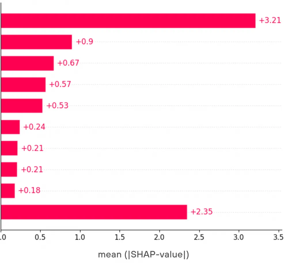
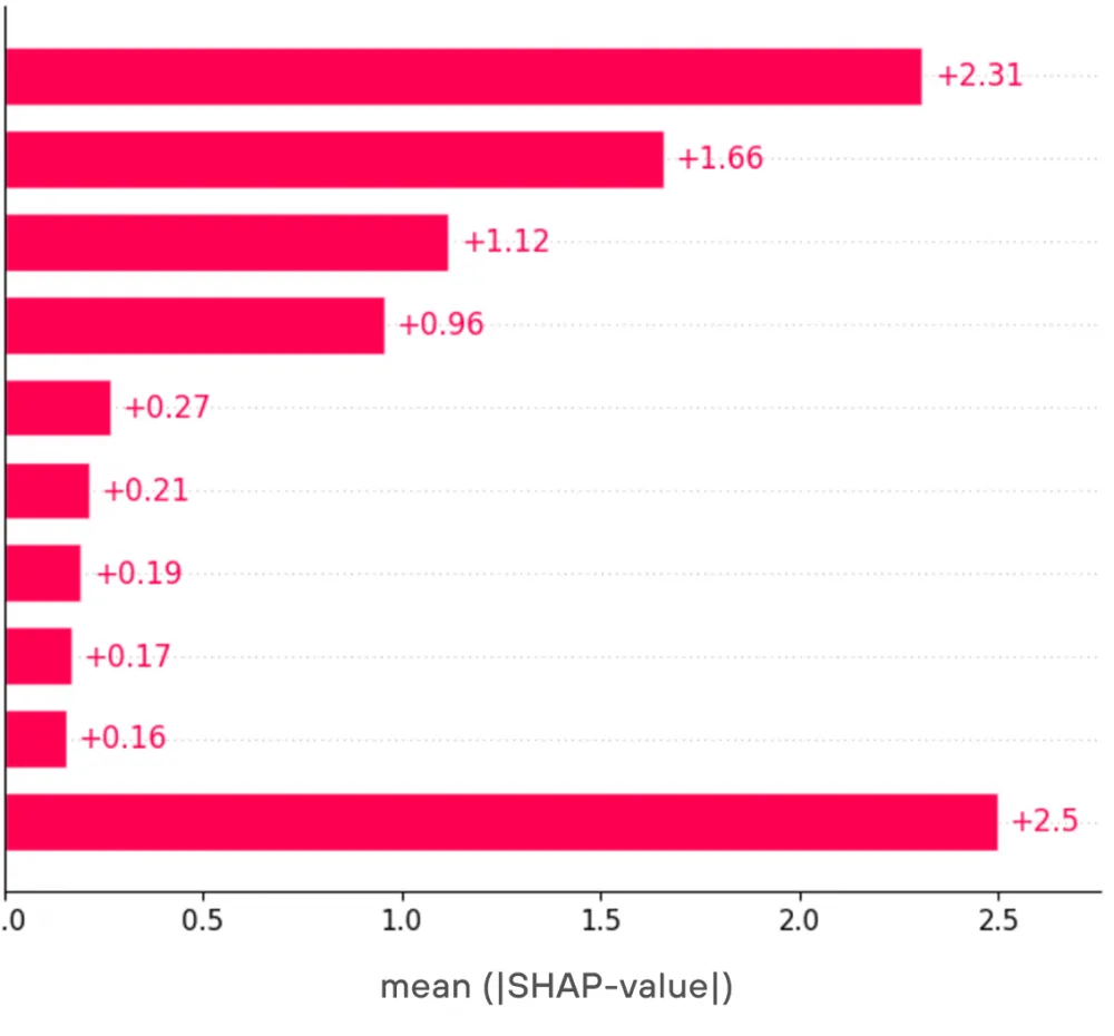
The last line indicates the overall contribution of all other features. As can be seen from the graph, through grouping, it was possible to slightly smooth the impact of features and add several new features that made a significant contribution to the model's verdicts.

Model quality after the update

At every step of our changes, we measured the quality on the validation sample, which was formed to be as close as possible to the data that our model might potentially encounter during inference.

Overall, as a result of all the aforementioned changes, we managed to improve the model's quality by ~12% (about an 8% increase in precision and about a 15% increase in F1-score).

However, since the model's release in the PT Sandbox, the validation sample is no longer a real indicator of quality but rather serves as a supportive tool for monitoring consecutive changes before the new version is released. Accordingly, the real metrics that interest us must be measured on real data from the model's performance in the product. Specifically, from a business value standpoint, the most important metric for us turned out to be the ratio of the number of unique detections by the model (when only this module was able to detect malicious activity among all product modules) to the number of false positives. Unique detections are very valuable, so an acceptable ratio is 1 to 2. This is the ratio we had at the time of the first version's product release. After all the consecutive changes, the model currently has a ratio close to 1 to 1.

It is worth noting that this ratio can be improved from two sides: by reducing false positives and by increasing the number of unique detections. The total number of model triggers will either decrease or increase accordingly. It is important to maintain a balance in these improvement options so that the model does not stop detecting new threats and successfully blocking them. We have been able to achieve this, as can be judged by specific cases that we discussed with our experts. More on this below.

Interesting findings, their behavior on the host and in traffic, and interpretation by the ML model

In our previous article, we already talked about the first network findings of the new software thanks to the ML model. However, by analyzing triggers in the flow and improving the feature set and their processing algorithm, we managed to discover many more interesting, and most importantly, previously undetectable samples. Below, we will share some of them (the most interesting ones)!

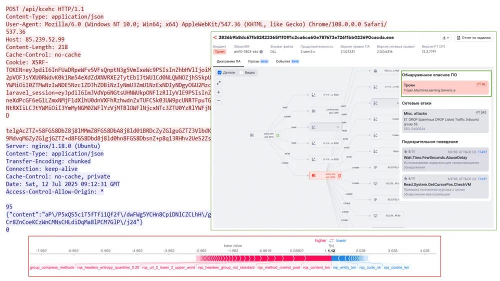
1. Backdoor Oyster — 3836b9b8dc67fb82423365f1f0ff1c2ca6ca60e787673e72611bb023690cacda

This backdoor was encountered a year ago, but this time the virus writers decided to evade detection and slightly changed the network interaction. Thanks to the activation of the ML model, we managed to detect a new version of Oyster and successfully identify it. As can be seen, the main triggers for the model in this case are the length of the request, the POST method, and an unconventional set of headers.

2. Loader (APT GOFFEE) — 2446f97c1884f70f97d68c2f22e8fc1b9b00e1559cd3ca540e8254749a693106

In the case of this loader from the COFFEE group (which we wrote about last summer), the model was able to identify its maliciousness thanks to a number of indicators, the most significant of which are the parameters in the URL request that transmit information about the system and user, as well as the small number and specific sequence of response headers.

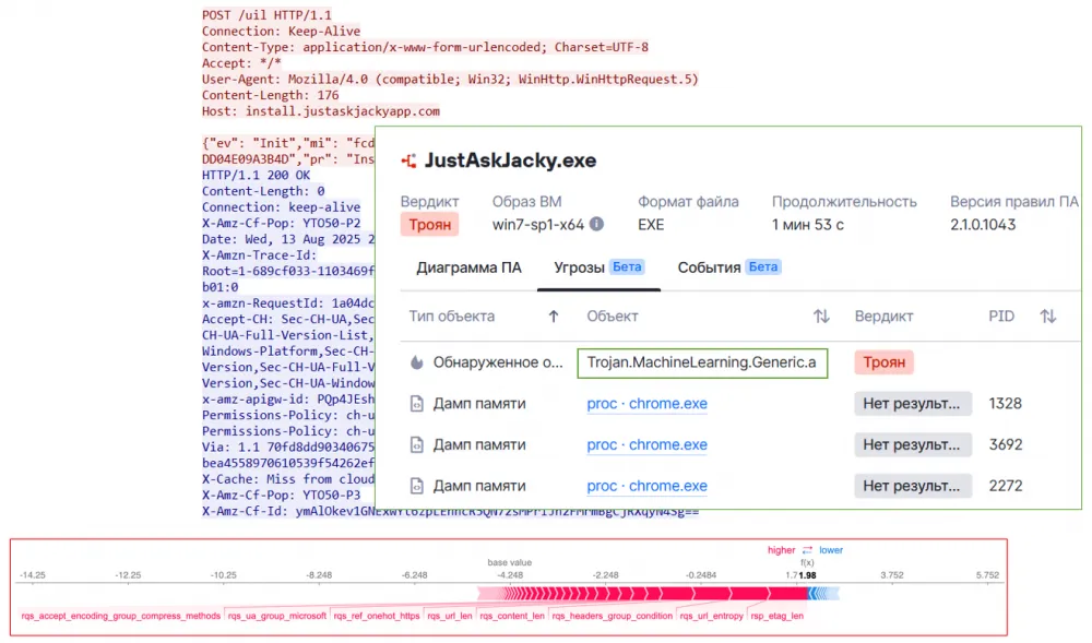
3. Stealer JustAskJacky — f05855fc1041a19649f2486ceb6a68b259d8969275f8ef455f17207f09be653b

For JustAskJacky, the verdict was signed by the outdated User-Agent, URL address, headers, and, of course, the body itself, which contains JSON with system data. By combining all this data, the ML model detected a previously undetectable stealer.

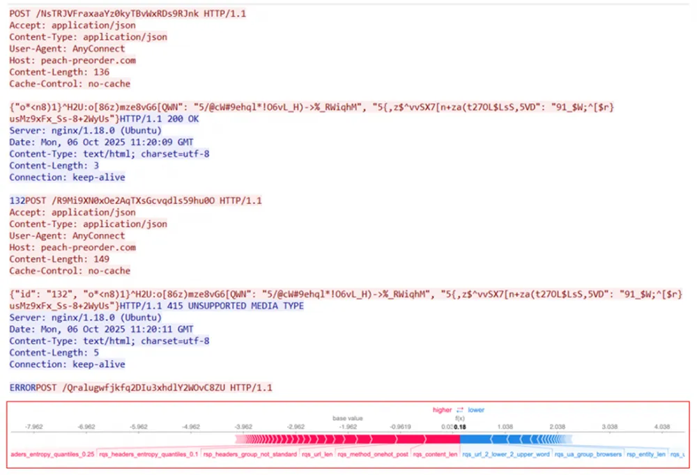
4. Stealer — f21483536cbd1fa4f5cb1e996adbe6a82522ca90e14975f6172794995ed9e9a2

As can be seen, this stealer forms a request with a rather specific URL string, and in the body, it transmits something clearly interesting — encrypted data about parameters and keys. The placement of headers and User-Agent also raises doubts about the legitimacy of this session. It is also worth noting that the server's response contains few headers and bytes in the body ("132" and "ERROR"). Thus, the ML model, by combining weights, marks this network interaction as "malicious" and turns out to be right.

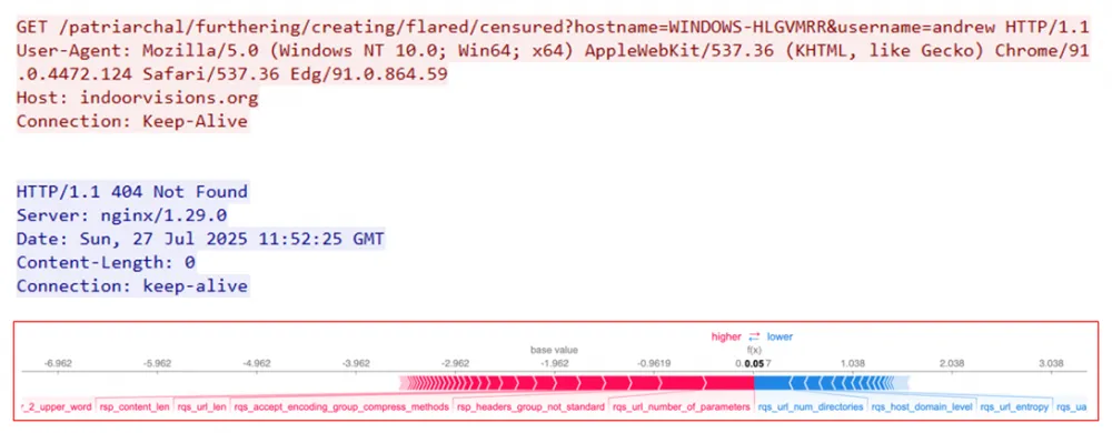
5. Loader — 6aa9e5d0b9da7582cea7768f5845e1446c1995df41531e3f31ca91bc6125ef4f

For this loader, brevity is the sister of talent, just as directness indicates that it has nothing to hide. Firstly, it specifies a unique key in UUID format in the URL, secondly, it explicitly states in the stage parameter that this is a loader, and finally, the small (only 3) number of request headers adds a bit more suspicion. Considering all these factors, which are quite uncharacteristic for legitimate sessions, we see how the ML model successfully detects a new threat again, which turns out to be unsuccessful in this case, as the server responds with 400 — something went wrong during the operation of the software vulnerability protection.

Conclusion

The ML model on HTTP requests greatly aids in analyzing samples in sandboxes, especially for malware that, after launch, does not reveal itself on the "compromised" host (does not try to inject into processes, register itself in registries, scan the file system and network interfaces, etc.), but simply communicates with C2 and waits for a response from the server. Often, such check-in requests change from sample to sample, which is why the machine learning model, due to its flexibility and the presence of fuzzy checks, helps to detect what signature checks might miss, and in our case, it does this excellently, as shown by the number of aforementioned findings!

Of course, we must reiterate that without specific content-containing rules, there is no escaping them; this is a foundation that, for better or worse, will remain in many information security tools for a long time. At the same time, ML is not a competitor to the well-established signatures but a helpful assistant that will uncover not only known threats but also new ones, which will ultimately enhance the detectability of malware across the entire product!

If you are interested in the process of building ML solutions in the field of cybersecurity and how new approaches to feature space can change the effectiveness of malware detection, stay with us and join the Telegram chat of the positivity ML team @falseposi.