Qucs-S: Guide to Simulation Types, Part 2

Temperature analysis (Temperature sweep)

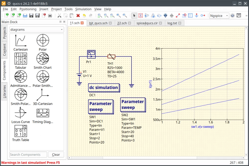
Temperature analysis is a type ofDC simulation. The difference is that you need to specify the TEMP variable, which is reserved for temperature in Ngspice, as a parameter. The screenshot shows an example of such a simulation. The dependence of the transistor collector current on temperature is simulated.

The following example illustrates the use of temperature in an external Parameter Sweep cycle. A circuit containing an NTC thermistor is simulated. This component is available in the Thermistor library supplied with the program.

Using equations with the Ngspice simulation engine

Equations are required either for creating parametric circuits or for manipulating simulation results. If the program is running in SPICE compatibility mode (by default), the use of equations has some peculiarities. Equations are divided into two types:

• Parameters (.PARAM) are calculated before simulation. As the name suggests, this type of equation is used for parametric circuits when it is necessary to calculate component values according to certain formulas. This type of equation is located on the left panel in the Equations group. For more details on the syntax, see the Ngspice manual: https://ngspice.sourceforge.io/docs/ngspice-html-manual/manual.xhtml#magicparlabel-1342

• Post-processor equations Nutmeg equation. These equations are calculated after simulation. Nutmeg is the scripting language of the Ngspice post-processor. This equation is placed on the circuit through the Insert→ Equation menu. For more details on Nutmeg: https://ngspice.sourceforge.io/docs/ngspice-html-manual/manual.xhtml#magicparlabel-24648

The peculiarity of Nutmeg equations is that they need to specify the type of simulation. This is due to the Ngspice syntax, in which it is impossible to distinguish the type of simulation.

• v(node) – voltage at a certain node of the circuit

• i(V1) current through the source

• V1#branch current through the source, obsolete syntax

Ngspice supports only currents through the source in equations. An expression like i(R1) results in an error. To measure the current through another component, it is necessary to connect a constant voltage source with zero voltage in series. The virtual ammeter available in Qucs-S is also a voltage source with zero voltage.

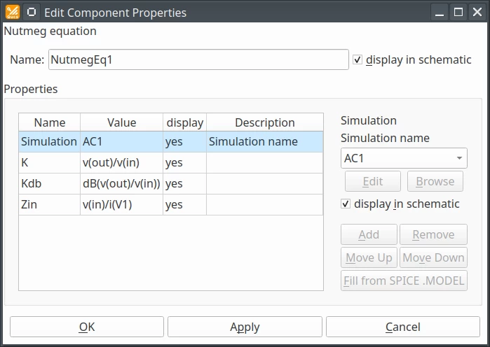
To bind the simulation to the Nutmeg equation, you can select it from the Simulation name drop-down list in the equation properties dialog as shown in the screenshot:

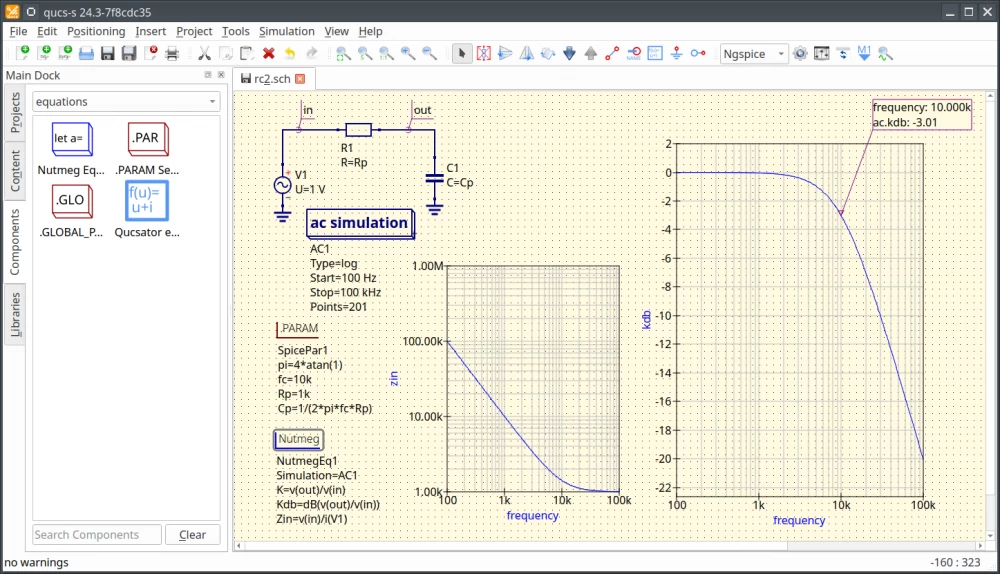
Let's consider an example. We will simulate an RC circuit such that the values of the capacitor and resistor are calculated based on the cutoff frequency (parameter fc). In the screenshot, we see that in addition to the circuit itself, AC1 simulation is set on the circuit field, and two equations are placed. The .PARAM parameter calculates the component values, and the Nutmeg Equation post-processor equation calculates the transfer coefficient K of the RC circuit and the input impedance Zin. This equation is bound to the AC1 simulation. The simulation results show that the cutoff frequency at the 3dB level is 10 kHz, as specified by the parameters.

Various mathematical functions can be used in Nutmeg equations. The full list can be found in the Ngspice documentation.

Using equations with the Qucsator simulation engine

Qucsator is not a SPICE-compatible engine and uses a different type of equations called Qucsator Equation. If Qucsator is selected as the default engine, this equation will be added to the circuit through a button on the toolbar.

Qucsator equations have a different syntax, not compatible with SPICE. The difference is that currents and voltages are uniquely determined. Therefore, it is not necessary to bind the simulation to the equation. Also, unlike SPICE, Qucsator is case-sensitive

• node.v – voltage at node during AC simulation

• node.V – voltage at node during DC simulation

• node.Vt – voltage at node during transient simulation

• V1.I – current through source V1 during DC simulation

• V1.i – current through source V1 during AC simulation

• V1.It – current through source V1 during transient simulation

• Pr1.It – current through virtual ammeter Pr1

• Pr1.Vt – voltage on virtual voltmeter Pr1

  Read also:

  • I waited 10 billion cycles and only got a loading screen

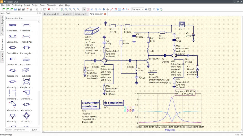
It should be noted that Qucsator has built-in functions for converting two-port network matrices. This is very convenient for analyzing microwave circuits. These functions should be used in conjunction with S-parameter simulation. Here are the main ones:

• stoz() converts S-parameter matrix to Z-parameter matrix

• stoy() converts S-parameter matrix to Y-parameter matrix

• rtoswr() converts reflection coefficient to VSWR

The screenshot shows an example of microwave amplifier simulation using equations.

More about Qucsator equations can be read in the manual from the old version of the program: https://qucs.sourceforge.net/docs/tutorial/getstarted.pdf The QucsatorRF engine supplied with Qucs-S is fully identical to the old version in terms of equation support.

Parametric Analysis (Parameter sweep) with Ngspice Engine

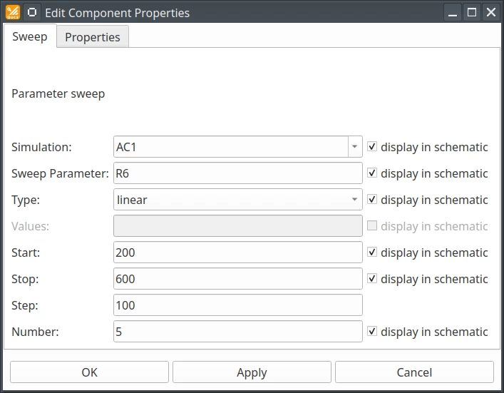
Parametric analysis is usually applied when it is necessary to obtain a family of graphs, for example, a family of frequency response curves, which depend on some parameter of the circuit. To use this type of modeling, the Parameter Sweep component should be placed on the circuit. In the properties dialog box of this type of modeling, you should specify the type of modeling to which the parameter sweep will be linked (Simulation dropdown list), as well as the parameter for the sweep (Sweep Parameter input field).

The following are allowed as parameters:

• Component name. Only resistor (R) or capacitor (C) is allowed.

• The name of a variable declared as a parameter (.PARAM)

To make the variable sweep work, Ngspice version newer than 37 is required. The screenshot shows an example of setting up a parametric analysis. AC1 is selected as the simulation, which should be placed on the circuit in advance. Resistor R6 is selected as the parameter for the sweep.

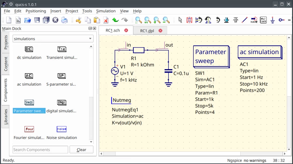
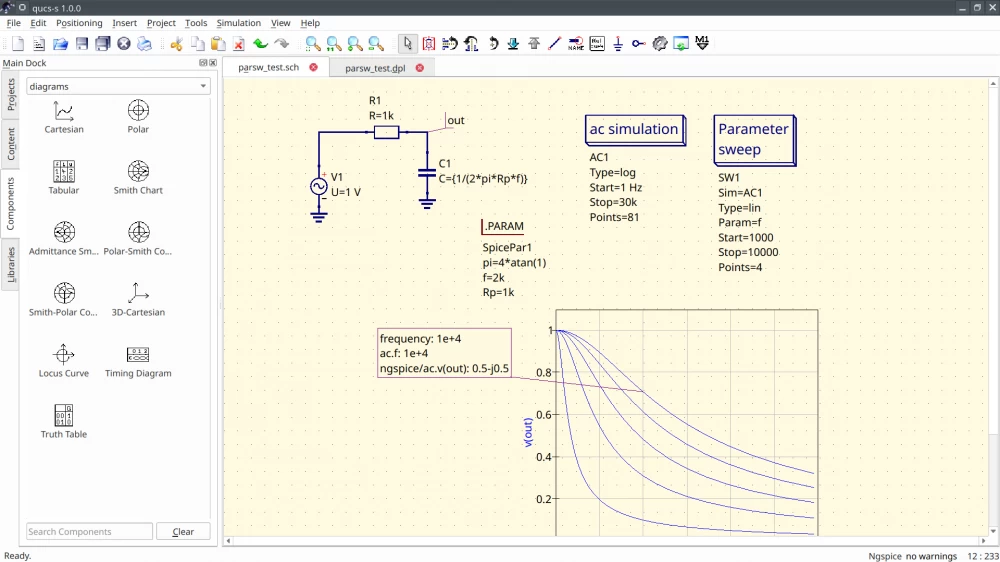
The following two screenshots illustrate examples of parametric analysis with a component as a parameter and a variable as a parameter. In the second example, the value of the capacitor in the RC circuit is calculated parametrically through a variable that sets the cutoff frequency. In both cases, as a result, we get a family of frequency response curves.

Zero-pole analysis

Zero-pole analysis allows you to calculate the location of zeros and poles of the transfer function on the complex plane. A brief theory on this issue can be found, for example, here: https://www.allaboutcircuits.com/technical-articles/understanding-poles-and-zeros-in-transfer-functions/ This modeling is used in the analysis of, for example, active filters in the frequency domain.

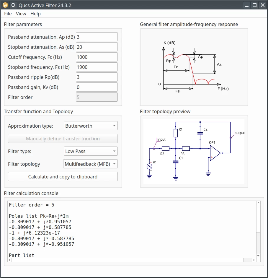
As an example, we synthesize a 5th-order Butterworth active filter using the built-in filter synthesis utility (Tools→ Active filter synthesis). We will select the initial data as shown in the screenshot. If you click the Calculate and copy to clipboard button, the synthesized circuit will be copied to the clipboard, and it can then be pasted into the document.

As a result of the calculation, the program, in addition to the nominal values of the elements, reports that the transfer function of the filter has 5 poles, which are symmetrically located on the complex plane. The program provides a normalized result for the unit cutoff frequency.

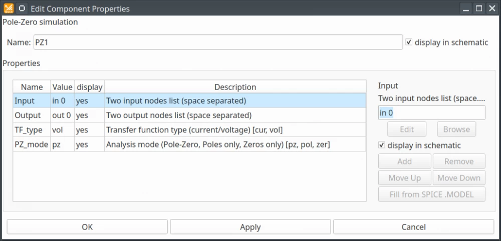
Let's simulate the placement of zeros and poles for this active filter. To do this, place the Pole/Zero analysis component on the circuit. In the properties, you need to specify a pair of input and output nodes. In our case, the input signal is applied between the nodes in and 0, and the output is taken between the nodes out and 0. Node 0 in SPICE-compatible simulators always corresponds to ground. Leave the other settings unchanged. The dialog box for the pole-zero analysis properties is shown in the following screenshot.

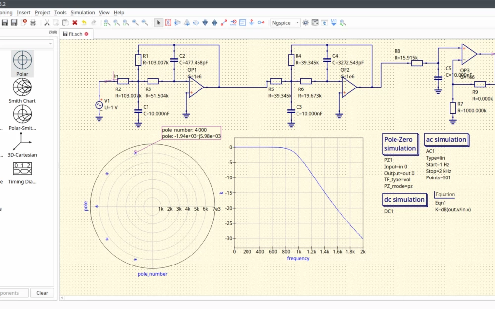
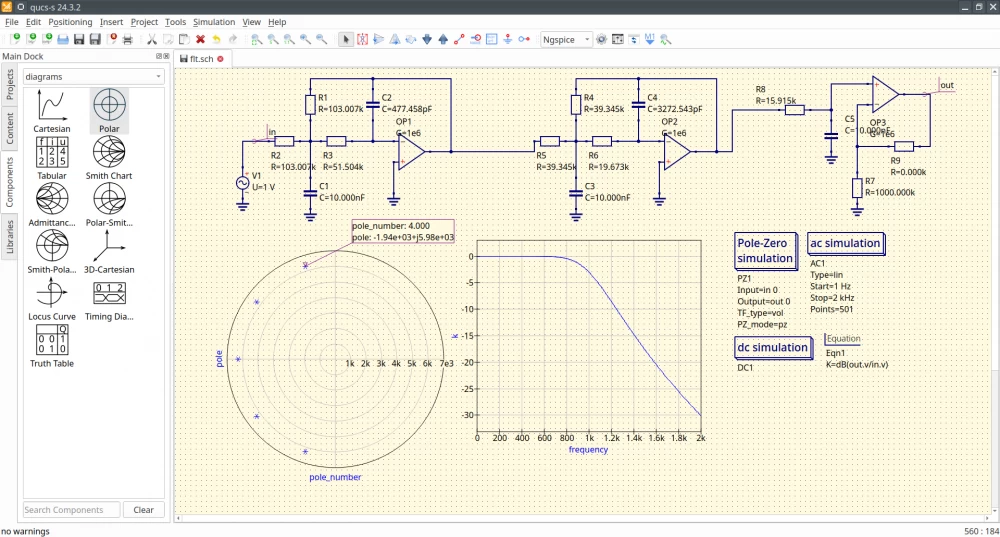
After the simulation, place a polar coordinate plot on the circuit and plot the pole variable. We get a plot of the pole locations on the complex plane. We also see five poles. In the diagram properties, you should specify the line type as stars. The numbers differ from the result in the previous screenshot. This is because the simulator outputs data multiplied by the cutoff circular frequency 2*pi*fc.

Conclusion

The first and second parts of the article cover most of the types of simulations available in Qucs-S. You can learn about the other types of simulations from the Ngspice documentation and the examples provided with the program. The conclusion provides a list of resources for Qucs-S.

• Project website: https://ra3xdh.github.io/

• Ngspice website: https://ngspice.sourceforge.io/

• Current release: https://github.com/ra3xdh/qucs_s/releases/tag/24.3.2

• Repository: https://github.com/ra3xdh/qucs_s

• Installation instructions: https://github.com/ra3xdh/qucs_s/wiki/Installation

• Forum: https://github.com/ra3xdh/qucs_s/discussions

• Bug tracker: https://github.com/ra3xdh/qucs_s/issues

• Boosty page where you can support the project financially: https://boosty.to/qucs_s